K = 2
ABSTAIN = -1

def lf_sentiment_words(text):
    text = text.lower()
    pos_count = sum(1 for w in ["great", "love", "amazing", "fun"] if w in text)
    neg_count = sum(1 for w in ["bad", "waste", "boring", "stupid"] if w in text)
    if pos_count > neg_count: return 1
    if neg_count > pos_count: return 0
    return ABSTAIN

def lf_viewing_experience(text):
    text_lower = text.lower()
    pos_watch = ["watched twice", "watch again", "rewatch", "couldn't stop watching"]
    neg_watch = ["walked out", "turned it off", "fell asleep", "couldn't finish"]
    pos = any(p in text_lower for p in pos_watch)
    neg = any(n in text_lower for n in neg_watch)
    if pos and not neg: return 1
    if neg and not pos: return 0
    return ABSTAIN

def lf_comparative_sentiment(text):
    text_lower = text.lower()
    if "worse than" in text_lower or "not as good as" in text_lower:
        return 0
return ABSTAINWeak Supervision
weak-supervision
machine-learning
data-labeling
Weak Supervision
Introduction
The idea behind weak supervision is that for each data point there is a latent true label that is inaccessible to us even during training, instead we utilize weak signals from user-defined labeling functions (LF). The material here is based on the data programming approach to weak supervision using LFs described in (Ratner et al. 2017). Here we extend to the multi-class case where the generative model has entries of the entire confusion matrix as learnable parameters.
LFs can be thought of as heuristic rules that can be applied to a large subset of the data. In case the LF is not applicable, then the function simply abstains from making a prediction. Note that this is a realistic scenario, it’s easier to describe rules than to manually annotate a large number of data points. LFs provide noisy, but potentially cost-effective labels, which can be used to train discriminative models.

Labeling Functions
Suppose we have a large corpus of text (e.g. the IMDB Movie Reviews dataset) that we want to classify as either positive or negative. Our goal is to predict labels for this dataset (with somewhat high accuracy) using only a minimal set of labeled examples. The ff. is an example of a positive movie review:
We always watch American movies with their particular accents from each region (south, west, etc). We have the same here. All foreign people must to watch this movie and need to have a open mind to accept another culture, besides American and European almost dominate the cinematographic industry.
This movie tell us about a parallel world which it isn’t figured even for those who live in a big city like São Paulo. All actors are improvising and they are very realistic. The camera give us an idea of their confuse world, the loneliness of each character and invite us to share their world.
It’s a real great movie and worst a rent even have it at home.
On the other hand, a negative movie review can look like:
I watch lots of scary movies (or at least they try to be) and this has to be the worst if not 2nd worst movie I have ever had to make myself try to sit through. I never knew the depths of Masacism until I rented this piece of moldy cheese covered in a used latex contraceptive. I am a fan of Julian Sans, but this is worse than I would hope for him.
On the other hand the story was promising and I was intrigued…for the first minute and a half while the credits rolled and I had yet to see what pain looked like first hand. Perhaps there are some viewers out there that enjoyed this and can point me in the right direction, but then again I know of those viewers who understand if not commemorate me, especially when we had to turn the video off, and that simply is NOT done with our watching (we had to make one exception obviously).
If it were up for a remake, I’d give it a chance so long as they had at most 1% of the original incorporated into it. That’s all.
Manually labeling thousands of reviews is expensive (and doesn’t scale well, i.e. linear), instead we can write heuristic rules called labeling functions (LF) primarily based on domain expertise or small observed examples. LFs scale well since it can be applied to a dataset in one sweep. Each LF inspects a review and returns 1 (positive), 0 (negative), or -1 (abstain). LFs can exploit many kinds of signals. Here we consider word counts, explicit ratings, viewing behavior, or comparative language:
Consider these example reviews and notice how each LF can be fooled or simply silent:
review = "I've watched this twice already and couldn't stop watching — the pacing is superb."

print(f"lf_sentiment_words        {str(lf_sentiment_words(review)):>2s}")          # abstain: no lexicon words match
print(f"lf_viewing_experience     {str(lf_viewing_experience(review)):>2s}")       # "couldn't stop watching" phrase present
print(f"lf_comparative_sentiment  {str(lf_comparative_sentiment(review)):>2s}")    # abstain: no comparative phrases match
lf_sentiment_words -1
lf_viewing_experience 1
lf_comparative_sentiment -1The ff. shows an issue with keyword matching where sense of negation is not captured (e.g. double negative):
review = "It's ok, not amazing but not worse than anything I've seen this year."

print(f"lf_sentiment_words        {str(lf_sentiment_words(review)):>2s}")          # captures "amazing" even when negated
print(f"lf_viewing_experience     {str(lf_viewing_experience(review)):>2s}")       # abstain: no viewing experience phrase present
print(f"lf_comparative_sentiment  {str(lf_comparative_sentiment(review)):>2s}")    # negative: "worse than" even if negated
lf_sentiment_words 1
lf_viewing_experience -1
lf_comparative_sentiment 0All abstain despite clear negative:
review = """
This movie is an absolute DISASTER. Two hours of my life I'll never get back.
The plot makes zero sense, the acting is wooden, and the dialogue sounds like
it was written by a toddler. Every scene drags on forever. I've seen better
cinematography in a high school project. The sound mixing is atrocious. Zero stars.
"""

print(f"lf_sentiment_words        {str(lf_sentiment_words(review)):>2s}")
print(f"lf_viewing_experience     {str(lf_viewing_experience(review)):>2s}")
print(f"lf_comparative_sentiment  {str(lf_comparative_sentiment(review)):>2s}")
lf_sentiment_words -1
lf_viewing_experience -1
lf_comparative_sentiment -1
Tip
LFs are iteratively refined in practice: we inspect disagreements between LFs, compare against any available ground truth, and consult domain knowledge. Since LFs are user-defined heuristics, they require some expertise and data exploration to be effective. This requires substantial effort and (from experience) can even be scoped as one project under a team of annotators.
Since human annotation and cross-checking multiple LF outputs is prohibitive, LLMs can also serve as LFs: instead of hand-writing heuristics, you prompt a model to generate heuristics for a labeling function. This is a form of knowledge distillation: the LLM’s broad world knowledge gets compressed into a smaller, faster model via the weak supervision pipeline rather than through soft targets directly. At the very extreme, an LLM itself can directly be an LF1:
def lf_llm(text):
    # can engineer abstention tendency by prompting
    response = client.chat.completions.create(...)
    return 1 if "positive" in response else 0 if "negative" in response else ABSTAIN
The generative model (discussed below) still earns its keep here, since LLM-based LFs can have systematic biases that confusion matrix estimation helps correct. Cost efficiency is the main motivation: pay for LLM inference on a small subset, then train on the full dataset using the resulting noisy labels. This can be more cost-effective over performing LLM inference at scale. Moreover, multiple LFs can be created from a single LLM by varying the prompt — different phrasings, chain-of-thought vs. few-shot, and so on, giving the model more signal to work with.
LF parameters
A labeling function is characterized by its coverage (fraction of inputs where it does not abstain) and its F1 score on non-abstaining inputs. For the IMDB task, our 20 LFs use diverse strategies — keyword matching, lexicon scoring, punctuation/structural heuristics, discourse patterns, and regex. A representative subset (calculated on actual data):
| LF | Strategy | Coverage | F1 |
|---|---|---|---|
lf_strong_sentiment |
keyword | 0.41 | 0.881 |
lf_sentiment_words |
keyword counting | 0.69 | 0.746 |
lf_lexicon_score |
scored lexicon | 0.45 | 0.790 |
lf_negation_density |
structural | 0.18 | 0.720 |
lf_sentence_sentiment |
sentence structure | 0.12 | 0.810 |
lf_comparative_regex |
regex | 0.08 | 0.850 |
lf_contrastive_but |
discourse | 0.15 | 0.740 |
There is a natural trade-off: LFs with broad coverage (like lf_sentiment_words) tend to have lower F1, while high-F1 LFs fire on fewer reviews (lf_strong_sentiment is a notable exception). The diversity of strategies ensures conditional independence — LFs based on different signals (structure, punctuation, lexicon, discourse) make mistakes on different subsets of the data. The full definitions of these LFs and their application to IMDB data appear in the application section at the end of this notebook.
Note
We generally do not have access to true labels for a representative sample of our dataset (or at best have access to a small labeled subset). Hence, even estimating the accuracy and coverage of our LFs is not possible. The following sections will deal with algorithms for estimating these parameters as well as training a machine learning model with noisy labels.
In practice, the generative model performs at roughly the F1 of the best LFs, modulated by their coverage. The ideal scenario is a set of conditionally independent LFs — ones that fire on different subsets of the data and make mistakes on different examples. In that case, the generative model can ensemble them toward higher F1 than any single LF alone, since other LFs compensate for the gaps of one.
Basic theory
For simplicity, we will limit our presentation to binary classification, although the method extends to the multiclass setting. For each data point \textbf{\textsf{x}} \in \mathcal{X}, the latent true label is y \in \mathcal{Y} = \{0, 1, \ldots, K-1\}. Suppose we have N labeling functions \lambda_j\colon \mathcal{X} \to \mathcal{Y} \cup \{-1\}, where -1 denotes abstention. Given M data points \textbf{\textsf{x}}_i, we obtain an M \times N matrix of LF outputs \Lambda_{ij} = \lambda_j(\textbf{\textsf{x}}_i).
We write \Lambda for the random variable representing LF outputs and \lambda_\textbf{\textsf{x}} for the realized output vector of a specific input. Our first step is to estimate the joint distribution p_\Phi(\lambda, y) as well as the marginal p_\Phi(\Lambda) = \prod_{i=1}^M p(\lambda_{\textbf{\textsf{x}}_i}). We do MLE to find parameters \hat{\Phi} that maximize the log-likelihood of the marginal p_\Phi(\Lambda) of the observed LF outputs. See below. This lets us calculate2:
\boxed{ p_{\hat{\Phi}}(y \mid \lambda_\textbf{\textsf{x}}) = \frac{p_{\hat{\Phi}}( y,\, \lambda_\textbf{\textsf{x}})}{p_{\hat{\Phi}}( \lambda_\textbf{\textsf{x}})} = \frac{p_{\hat{\Phi}}( \lambda_\textbf{\textsf{x}} \mid y)\, p_y}{\sum_{y'=0}^{K-1} p_{\hat{\Phi}}(\lambda_\textbf{\textsf{x}} \mid y')\, p_{y'}} }
for any y = 0, \ldots, K-1 and any input \textbf{\textsf{x}}. Given this, we perform noise-aware training (NAT) of a classifier f_\Theta by minimizing the following loss:
\boxed{ \mathcal{L}_{\text{NAT}}(\Theta) = -\frac{1}{M}\sum_{i=1}^M \sum_{y=0}^{K-1} {p_{\hat{\Phi}}(y \mid \lambda_{\textbf{\textsf{x}}_i})} \cdot \log \text{Softmax}(f_\Theta(\textbf{\textsf{x}}_i))_y }
where the sum over y is the soft cross-entropy loss. This looks like the usual loss, except we don’t have a single label. All labels contribute weighted by the probability of the label given the LF outputs of the input. The key insight is that the generative model is blind to the input features \textbf{\textsf{x}} — it only sees LF outputs. Hence, we train on every candidate label, using the posterior p_{\hat{\Phi}}(y \mid \lambda_{\textbf{\textsf{x}}_i}) to steer how much each contributes to the gradient. As training progresses, f_\Theta learns feature-to-label mappings that are simultaneously good classifiers and consistent with the LF-derived posterior — becoming confident on inputs where the generative model alone cannot be.
Note
Each combination of N LF outputs defines one of 3^N patterns, and the generative model assigns the same soft label to all points sharing a pattern. Exponential growth helps: 7 LFs yield 3^7 = 2{,}187 bins. So this discretizes the space, and we rely on the hypothesis that points in the same bin share a label distribution for sufficiently large N (which we hope to be not too large).
Generative model
Each LF has its own confusion matrix showing how its outputs relate to the true labels. For instance, lf_sentiment_words has asymmetric accuracy — it is much better at identifying positive reviews than negative ones:
import numpy as np
import pandas as pd
from datasets import load_dataset

from notebooks.utils import set_seed

RANDOM_SEED = 0
set_seed(RANDOM_SEED)

ds = load_dataset("imdb")["train"].shuffle(seed=RANDOM_SEED).select(range(1000))
ds_texts = ds["text"]
ds_label = ds["label"]  # {0, 1}
Example confusion matrix for one LF:
from sklearn.metrics import confusion_matrix as cm

y = np.array(ds_label)
out = np.array([lf_sentiment_words(t) for t in ds_texts])
F = out != ABSTAIN
label = y[F]
preds = out[F]

conf = cm(label, preds, labels=[0, 1])
df = pd.DataFrame(conf, index=["y=0 (neg)", "y=1 (pos)"], columns=["pred=0", "pred=1"])
df["abstain"] = [sum(y[~F] == 0).item(), sum(y[~F] == 1).item()]
df| pred=0 | pred=1 | abstain | |
|---|---|---|---|
| y=0 (neg) | 166 | 135 | 206 |
| y=1 (pos) | 25 | 291 | 177 |
Observe that this can be converted to conditional probabilities given y. Let’s call the resulting matrix \mathbf{C}^{(j)} \in [0, 1]^{K \times (K + 1)}:
df / df.sum(axis=1).values.reshape(-1, 1)| pred=0 | pred=1 | abstain | |
|---|---|---|---|
| y=0 (neg) | 0.327416 | 0.266272 | 0.406312 |
| y=1 (pos) | 0.050710 | 0.590264 | 0.359026 |
This is precisely what the generative model will learn from input data. To see this, consider an input \textbf{\textsf{x}}, we get LF outputs \lambda_\textbf{\textsf{x}} \in [-1, 0, \ldots, K-1]^N. The marginal probability of this output vector is then:
\boxed{p(\lambda_\textbf{\textsf{x}} ) = \sum_y p_{y} \cdot p_{{\Phi}}(\lambda_\textbf{\textsf{x}} \mid y) = \sum_{y} p_y \cdot \prod_j C^j_{y, \lambda_j}}.
Here we have to provide the prior distribution since the labels are censored. Also, we assume that the LF outputs are conditionally independent given the true label. Note that the rows of \mathbf{C}^{j} sum to 1, so our network will have logits of shape K \times (K + 1) with entries ranging over \mathbb{R}; we later apply softmax along the rows. Finally, our goal is to perform MLE on \Phi = \{\mathbf{C}^1, \ldots, \mathbf{C}^N\} by minimizing over the dataset:
\boxed{ \mathcal{L}_{\text{gen}}(\Phi) = \frac{1}{M}\sum_{i=1}^M -\log \left( \sum_{y=0}^{K-1} p_y \cdot \prod_{j=1}^N C^j_{y,\, \Lambda_{ij}} \right) }.
Note
Why model p(\Lambda \mid Y) rather than p(Y \mid \Lambda) directly? Because the forward direction — how each LF behaves given a true label — is what we can decompose per-LF and estimate from unlabeled data. Each LF has its own confusion matrix independent of the others. Bayes’ rule then gives us the posterior we actually need.
Tip
In practice, to avoid underflow with large number of LFs, we implement this using the \text{LogSumExp} trick (e.g. with torch.logsumexp) as:
{\log p(\lambda_\textbf{\textsf{x}}) = \log \sum_y \exp\!\left(\log p_y + \sum_j \log C^j_{y,\,\lambda_j}\right)}
so that
{ \mathcal{L}_{\text{gen}}(\Phi) = -\frac{1}{M}\sum_{i=1}^M \log \sum_{y=0}^{K-1} \exp\!\left(\log p_y + \sum_{j=1}^N \log C^j_{y,\,\Lambda_{ij}}\right) }.
Finally, the soft target probability is given by:
{ p_{\hat{\Phi}}(y \mid \lambda_\textbf{\textsf{x}}) = \exp\Bigg(\log p_y + \sum_j \log C^j_{y,\,\lambda_j} - \log \sum_{y'} \exp\!\left(\log p_{y'} + \sum_j \log C^j_{y',\,\lambda_j}\right)\Bigg). }
Code implementation
For convenience, we let the elements of \mathbf{C}^j be real numbers. Then, for each j, the confusion matrix of the LF is obtained by taking the softmax along dim=1 (i.e. conditioned on the target which is indexed in dim=0). We stack these along the third dimension so that we get a tensor \mathbf{C} of shape (K, K + 1, N). Since softmax is shift-invariant, we can initialize the abstain logits as C_{y, K} = 0 for all y, and derive its value from non-abstain logits. This also makes it explicit that we have K free parameters along a row.
import torch
torch.manual_seed(1)

K = 2
n = 4

# C[y, k, j] := P(λ_j = k | Y = y)
# C_logits is the unnormalized log-probs, which we optimize with gradient descent.
C_logits = torch.randn(K, K + 1, n)
C_logits[:, -1, :] = 0
C = torch.softmax(C_logits, dim=1)

print("Confusion matrix shape:", C.shape)
print(C)
print(C.sum(dim=1).numpy().sum())   # ~8 (2 targets x 4 LFs)
Confusion matrix shape: torch.Size([2, 3, 4])
tensor([[[0.1025, 0.2342, 0.2743, 0.1428],
[0.4263, 0.2697, 0.1981, 0.1429],
[0.4712, 0.4960, 0.5276, 0.7143]],
[[0.4422, 0.0792, 0.2385, 0.1015],
[0.1731, 0.5370, 0.4328, 0.7616],
[0.3847, 0.3838, 0.3287, 0.1369]]])
8.0We index into the confusion matrix using the LF output matrix. Class labels \{0, \ldots, K-1\} map to the first K columns, and abstain (K) maps to the last column. No remapping needed:
# Example LF output matrix: values in {0, 1, ..., K} where K = abstain
L = torch.tensor([
    [0, K,  1,  1],
    [1, 0,  0,  K],
])

# P(L | y=1): for each instance i and LF j, look up C[y=1, L[i,j], j]
y = 1
C[y, L, torch.arange(n)]  # shape: (m, n)
tensor([[0.4422, 0.3838, 0.4328, 0.7616],
[0.1731, 0.0792, 0.2385, 0.1369]])The product across LFs gives the conditional likelihood of the observed LF outputs for a given true label:
# P(Λ_i | y) = prod_j C[y, Λ_{ij}, j]
for y in range(K):
    probs = C[y, L, torch.arange(n)]  # (m, n)
    print(f"P(Λ | y={y}):", probs.prod(dim=1))
P(Λ | y=0): tensor([0.0014, 0.0196])
P(Λ | y=1): tensor([0.0560, 0.0004])The marginal probability of the two LF outputs over the latent label:
py = torch.tensor([0.5, 0.5])  # class prior

p_marginal = sum(
    py[y] * C[y, L, torch.arange(n)].prod(dim=1)
    for y in range(K)
)

print("P([Λ0, Λ1]):", p_marginal)
P([Λ0, Λ1]): tensor([0.0287, 0.0100])Finally, the marginal probability of the sample p_{\Phi}(\Lambda). Because we generally have M \gg 1 terms with values in [0, 1], we use \log to avoid underflow:
print("     p(Λ):", p_marginal.prod().item())
print("-log p(Λ):", -torch.log(p_marginal).sum().item())
p(Λ): 0.00028718687826767564
-log p(Λ): 8.155377388000488Demo experiments
from tqdm.notebook import tqdm
import matplotlib.pyplot as plt
from notebooks.plot import set_format

set_format("svg")
set_seed(RANDOM_SEED)
Simulated LFs
Generating a toy dataset. Also setting the prior label probabilities:
m = 10000
K = 2
LABEL_PROBS = {0: 0.40, 1: 0.60}
y_true = np.random.choice([0, 1], size=m, p=[LABEL_PROBS[0], LABEL_PROBS[1]])

s = 2 * torch.pi * torch.rand(m, 1)
r = 0.5 * torch.tensor(y_true, dtype=torch.float32).view(-1, 1)  # 0 -> r=0, 1 -> r=0.5
x = torch.cat([r * torch.cos(s), r * torch.sin(s)], dim=1) + 0.05 * torch.randn(m, 2)

t = np.linspace(0, 2*np.pi, 100)
x0 = 0.5 * np.cos(t)
x1 = 0.5 * np.sin(t)
x_neg = x[torch.where(torch.tensor(y_true) == 0)]
x_pos = x[torch.where(torch.tensor(y_true) == 1)]
Code
def plot_dataset(x_neg, x_pos):
    m = len(x_neg)
    limit = m // 10
    plt.figure(figsize=(6, 3))
    plt.scatter(x_neg[:limit, 0], x_neg[:limit, 1], s=10.0, edgecolor="k", color="C0", label="y = 0")
    plt.scatter(x_pos[:limit, 0], x_pos[:limit, 1], s=10.0, edgecolor="k", color="C1", label="y = 1")
    plt.plot(x0, x1, color='black', linewidth=1, linestyle='dashed', label="r = 0.25")
    plt.xlabel("x$_0$")
    plt.ylabel("x$_1$")
    plt.legend()
    plt.axis("equal")

plot_dataset(x_neg, x_pos)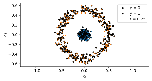
Figure. Below we use r = 0.25 as basis for synthetic LFs.
Note that radius less than 0.25 determines the label as y = 0 (with high probability):
# radius >= 0.25 -> class 1, else class 0
((torch.sqrt((x ** 2).sum(dim=1)) >= 0.25).long().numpy() == y_true).mean()np.float64(1.0)We use this to write simulated LFs with given parameters:
def lf_sim(coverage, accuracy):
    def predict(x):
        m = x.shape[0]
        y = (torch.sqrt((x ** 2).sum(dim=1)) >= 0.25).long()  # 0 or 1
        abstain_mask = torch.rand(m) >= coverage
        flip_mask = torch.rand(m) >= accuracy
        y[flip_mask] = 1 - y[flip_mask]         # flip label
        y[abstain_mask] = ABSTAIN               # -1
        return y
    return predict

# example
p = lf_sim(0.3, 0.8)(x).numpy()
fired = p != ABSTAIN
print("cov: ", fired.mean())
print("acc: ", (p[fired] == y_true[fired]).mean())
print("acc (y=0):", (p[fired & (y_true == 0)] == y_true[fired & (y_true == 0)]).mean())
print("acc (y=1):", (p[fired & (y_true == 1)] == y_true[fired & (y_true == 1)]).mean())
cov: 0.2993
acc: 0.7945205479452054
acc (y=0): 0.7960848287112561
acc (y=1): 0.7934352009054896Initializing the empirical LF matrix for display. Some LFs have fairly low F1 on their covered examples:
lf_params = [(0.30, 0.75), (0.50, 0.65), (0.40, 0.70), (0.20, 0.80), (0.25, 0.90)]
labeling_funcs = [lf_sim(*param) for param in lf_params]

df = pd.DataFrame({"y": y_true})
df["x0"] = x[:, 0].numpy()
df["x1"] = x[:, 1].numpy()
for j, lf in enumerate(labeling_funcs):
    df[f"LF{j + 1}"] = lf(x).int().numpy()

print(df.shape)
df.head()
(10000, 8)| y | x0 | x1 | LF1 | LF2 | LF3 | LF4 | LF5 | |
|---|---|---|---|---|---|---|---|---|
| 0 | 1 | -0.599245 | 0.044822 | -1 | 1 | -1 | -1 | -1 |
| 1 | 1 | 0.045224 | -0.489432 | -1 | -1 | 0 | -1 | -1 |
| 2 | 1 | 0.367845 | 0.195856 | -1 | 1 | 0 | 1 | -1 |
| 3 | 1 | 0.345199 | 0.440180 | -1 | -1 | -1 | -1 | -1 |
| 4 | 1 | -0.138734 | 0.433529 | 1 | 1 | -1 | -1 | -1 |
Data split and LF matrix. We split the data 80-20 for evaluation and precompute the LF output matrix \Lambda for each split. Since lf_sim is stochastic (each call generates a fresh random sample), we call each LF once per split and store the results:
# 80-20
SPLIT_RATIO = 0.80
m = x.shape[0]

x_train = x[:int(SPLIT_RATIO * m)]
x_valid = x[int(SPLIT_RATIO * m):]
y_train = torch.tensor(y_true[:int(SPLIT_RATIO * m)])
y_valid = torch.tensor(y_true[int(SPLIT_RATIO * m):])

def build_L(labeling_funcs, x):
    """Build LF output matrix from labeling functions. Shape: (m, N)."""
    return torch.stack([lf(x) for lf in labeling_funcs], dim=1).long()

L_train = build_L(labeling_funcs, x_train)
L_valid = build_L(labeling_funcs, x_valid)
print(f"L_train: {L_train.shape}, L_valid: {L_valid.shape}")
L_train: torch.Size([8000, 5]), L_valid: torch.Size([2000, 5])Generative model training
We implement GenModel as a predicting posterior probability of each class given LF outputs.
Note
We train the generative model with SGD and full-batch gradient descent. The logits are warm-started with a diagonal preference (logits[y, y, :] += 1.0) to encourage the model to assign higher probability to the correct class initially. This bias resulted in significantly better performance.
class Predictor:
    def __init__(self, clf, num_classes: int, output_probs=False):
        self.clf = clf
        self.K = num_classes
        self.output_probs = output_probs

    @torch.no_grad()
    def predict_proba(self, x):
        out = self.clf(x)
        return out if self.output_probs else torch.softmax(out, dim=1)

    @torch.no_grad()
    def predict(self, x, t=None):
        """Predict labels. For binary, threshold t on y=1 can be used."""
        probs = self.predict_proba(x)
        if t is not None and self.K == 2:
            return (probs[:, 1] >= t).long()
        return probs.argmax(dim=1)


class GenModel(Predictor):
    def __init__(self, num_classes: int, num_lfs: int, class_prior: dict = None):
3        super().__init__(self, num_classes, output_probs=True)
        self.N = num_lfs
        self.K = num_classes
        self.output_probs = True
        py = [1.0 / self.K] * self.K if class_prior is None else [class_prior[k] for k in range(self.K)]
        self.py = torch.tensor(py, dtype=torch.float32)  # shape (K,)

1        logits = 0.1 * torch.randn(self.K, self.K, self.N)
        logits[range(self.K), range(self.K), :] += 1.0
        self.logits = torch.nn.Parameter(logits)

    @property
    def C(self):
        zeros = torch.zeros(self.K, 1, self.N, device=self.logits.device)
        return torch.softmax(torch.cat([self.logits, zeros], dim=1), dim=1)

    def fit(self, L_train, L_valid=None, epochs=1, lr=0.01):
        """MLE estimate of confusion matrix parameters."""

2        optimizer = torch.optim.Adam([self.logits], lr=lr)
        history = {"train": [], "valid": [], "valid_steps": []}
        checkpoint = (None, np.inf)

        try:
            for e in tqdm(range(epochs)):
                loss = self.loss_fn(L_train)
                optimizer.zero_grad()
                loss.backward()
                optimizer.step()
                history["train"].append(loss.item())

                with torch.no_grad():
                    if L_valid is not None:
                        val_loss = self.loss_fn(L_valid)
                        history["valid"].append(val_loss.item())
                        history["valid_steps"].append(e + 1)
                        if val_loss.item() < checkpoint[1]:
                            checkpoint = (self.logits.detach().clone(), val_loss.item())

        except KeyboardInterrupt:
            print("Training stopped.")

        except Exception as e:
            print("An error occurred during training:", str(e))

        finally:
            # Load best model from checkpoint; freeze for inference
            self.logits = checkpoint[0]
            history["best_val_loss"] = checkpoint[1]
            return history

    def predict_log_joint_proba(self, L):
        """Estimate log p(Λ_i, Y=y) for each instance. Shape: (M, K)."""
        n = L.shape[1]
        k = self.K
        log_py = self.py.view(k, -1).log()
        return (log_py + self.C[:, L, torch.arange(n)].log().sum(dim=2)).T

    def loss_fn(self, L):
        log_p_joint = self.predict_log_joint_proba(L)
        return -torch.logsumexp(log_p_joint, dim=1).mean()

    def predict_log_proba(self, L):
        """Estimate log p(Y=y | Λ) via Bayes' rule. Shape: (M, K)."""
        log_p_joint = self.predict_log_joint_proba(L)
        return log_p_joint - torch.logsumexp(log_p_joint, dim=1, keepdim=True)

    def __call__(self, L):
        """Estimated posterior probs p(Y=y | Λ) via Bayes' rule. Shape: (M, K)."""
        return self.predict_log_proba(L).exp()


set_seed(RANDOM_SEED)

N = L_train.shape[1]
gen_model = GenModel(num_classes=K, num_lfs=N, class_prior=LABEL_PROBS)
history = gen_model.fit(L_train, L_valid, epochs=1000, lr=0.03)- 1
- Logits are initialized to have 0.1 variance, with diagonal entries shifted by +1.
- 2
- Adam on full batch with the LF confusion parameters. Since the model is simple there is no benefit to adding noise with SGD, and we simply try to overfit on the LF outputs. The curve below validates this hypothesis.
- 3
-
Setting
clfasselfinPredictorinit withoutput_probs=True. Hence, we have to define a__call__method that outputs probabilities.
seed: 0 deterministic: FalseCode
plt.figure(figsize=(6, 3))
plt.plot(history["train"], label="train")
plt.plot(history["valid_steps"], history["valid"], label="valid")
plt.ylabel("loss")
plt.xlabel("epoch")
plt.legend()
plt.grid(linestyle="dotted", alpha=0.6)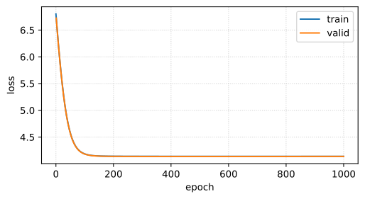
The model recovers the latent LF parameters better when coverage is high. Low-coverage LFs have fewer observed (non-abstain) outputs, making their confusion matrices harder to estimate:
from sklearn.metrics import f1_score

def estimated_f1(gen_model, j, p_classes):
    cm = gen_model.C[:, :, j].numpy()
    c = cm[:, :-1] * p_classes.reshape(-1, 1)
    precision = c[1, 1] / c[:, 1].sum()
    recall = c[1, 1] / c[1, :].sum()
    f1 = 2 * (precision * recall) / (precision + recall)
    return f1

def estimated_cov(gen_model, j, p_classes):
    cm = gen_model.C[:, :, j].numpy()
    learned_cov = cm[:, -1]
    return (1 - (learned_cov * p_classes).sum()).item()

rows = []
p_classes = np.array(list(LABEL_PROBS.values()))
for j in range(len(lf_params)):
    est_cov = estimated_cov(gen_model, j, p_classes)
    est_f1 = estimated_f1(gen_model, j, p_classes)
    mask = L_train[:, j] != ABSTAIN
    emp_f1 = f1_score(L_train[mask, j], y_train[mask]) # empirical F1

    rows.append({
        "lf":         f"LF{j+1}",
        "latent cov": lf_params[j][0],
        "est cov":    round(est_cov, 2),
        "latent F1":  round(emp_f1, 2),
        "est F1":     round(est_f1, 2),
    })

pd.DataFrame(rows).set_index("lf")| latent cov | est cov | latent F1 | est F1 | |
|---|---|---|---|---|
| lf | ||||
| LF1 | 0.30 | 0.30 | 0.78 | 0.80 |
| LF2 | 0.50 | 0.49 | 0.69 | 0.68 |
| LF3 | 0.40 | 0.40 | 0.74 | 0.74 |
| LF4 | 0.20 | 0.20 | 0.82 | 0.80 |
| LF5 | 0.25 | 0.25 | 0.92 | 0.88 |
Code
from notebooks.plot import Plot

# Create a plot
p = Plot(1, len(labeling_funcs), figsize=(8.5, 2))

for j in range(len(labeling_funcs)):
    p[j].heatmap(
        torch.softmax(gen_model.C[:, :, j], dim=1),
        row_labels=["y=0", "y=1"],
        col_labels=["pred=0", "pred=1", "pred=-1"],
        cmap="Blues",
        fmt=".2f",
        colorbar=False
    )
    p[j].labels(title=f"LF{j + 1}")
p.show()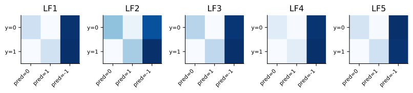
Code
frames = []
for j in range(len(lf_params)):
    C_j = gen_model.C[:, :, j]
    df = pd.DataFrame(
        C_j.numpy(),
        index=pd.MultiIndex.from_tuples([(f"LF{j+1}", f"y={k}") for k in range(K)]),
        columns=[f"pred={k}" for k in range(K)] + ["abstain"]
    )
    frames.append(df)
pd.concat(frames)| pred=0 | pred=1 | abstain | ||
|---|---|---|---|---|
| LF1 | y=0 | 0.235353 | 0.065865 | 0.698783 |
| y=1 | 0.067697 | 0.224783 | 0.707519 | |
| LF2 | y=0 | 0.325458 | 0.190916 | 0.483626 |
| y=1 | 0.166631 | 0.307072 | 0.526297 | |
| LF3 | y=0 | 0.286357 | 0.117871 | 0.595771 |
| y=1 | 0.117910 | 0.274488 | 0.607602 | |
| LF4 | y=0 | 0.163372 | 0.047947 | 0.788681 |
| y=1 | 0.042908 | 0.153785 | 0.803307 | |
| LF5 | y=0 | 0.203996 | 0.040648 | 0.755356 |
| y=1 | 0.032851 | 0.225140 | 0.742010 |
The trained model can be used to estimate conditional probabilities of targets given LF outputs:
# Simple test that the model learned (without using latent labels):
l = torch.tensor([[1, 1, 1, 1, 1]])
for y in range(K):
    print(f"p(y={y} | Λ=all_pos): {gen_model.predict_proba(l)[0, y].item():.4f}")

print()
l = torch.tensor([[0, 0, 0, 0, 0]])
for y in range(K):
    print(f"p(y={y} | Λ=all_neg): {gen_model.predict_proba(l)[0, y].item():.4f}")
p(y=0 | Λ=all_pos): 0.0029
p(y=1 | Λ=all_pos): 0.9971
p(y=0 | Λ=all_neg): 0.9962
p(y=1 | Λ=all_neg): 0.0038The conditional probabilities of targets given LF outputs sum to 1 (passes sanity check).
l = torch.tensor([[-1, -1, -1, -1, -1]])
for y in range(K):
    print(f"p(y={y} | Λ=all_abstain): {gen_model.predict_proba(l)[0, y].item():.4f}")
p(y=0 | Λ=all_abstain): 0.3722
p(y=1 | Λ=all_abstain): 0.6278
Note
When all LFs abstain, the posterior is:
p(y \mid \text{all abstain}) = \frac{p_y \cdot \prod_j C^j_{y,\,K}}{\sum_{y'} p_{y'} \cdot \prod_j C^j_{y',\,K}}
This only equals the prior p_y if \prod_j C^j_{y,K} is the same for all y — i.e., the joint abstention rate is class-independent. In general it’s not exactly the prior; the abstain column of each confusion matrix can differ across rows, so even “all abstain” carries some signal about y.
That said, in practice abstention rates are often similar across classes (an LF fires on surface patterns, not the true label directly), so the posterior approximately collapses to the prior. And conceptually this makes sense: if no LF speaks up, the best you can do is fall back on your base rate.
Label inference (binary)
Soft labels can be generated for a test input using p_{\hat{\Phi}}(y \mid \lambda_\textbf{\textsf{x}}) calculated using learned LF parameters. This already takes into account the prior label distribution. In particular, if all LFs abstain, then the model falls back roughly to the prior label distribution (see above note). Evaluating by means of ground truth labels:
import warnings
warnings.filterwarnings("ignore")

from sklearn.metrics import (
    f1_score,
    confusion_matrix,
    precision_score,
    recall_score
)

def evaluate(model, x, y, t=0.5, verbose=True):
    m = x.shape[0]
    preds = model.predict(x, t)
    f1 = f1_score(y.numpy(), preds.numpy(), average="weighted")
    recall = recall_score(y.numpy(), preds.numpy(), average="weighted")
    precision = precision_score(y.numpy(), preds.numpy(), average="weighted")

    if verbose:
        print(confusion_matrix(y.numpy(), preds.numpy()))

    return {
        "f1": f1,
        "recall": recall,
        "precision": precision,
        "m": m, "message": f"m={m}, f1={f1:.5f}, t={t:.5f}"
    }

# Since data is imbalanced t=0.5 can be suboptimal (assuming calibrated probs)
t_cal = torch.quantile(gen_model.predict_proba(L_train)[:, 1], q=LABEL_PROBS[0])
print(evaluate(gen_model, L_train, y_train, t=t_cal)["message"]); print()
print(evaluate(gen_model, L_valid, y_valid, t=t_cal)["message"])
[[2220 1023]
[ 946 3811]]
m=8000, f1=0.75338, t=0.62777
[[554 232]
[220 994]]
m=2000, f1=0.77369, t=0.62777
Tip
Matching the label prior distribution. The threshold for predicting hard labels can be calibrated by using the prior label distribution. Let \pi = p_1. We want: \textrm{P}(f(x) \geq t)=\pi which implies \textrm{P}(f(x)<t)=1-\pi. This is exactly what a q-quantile gives: the value below which fraction q of data lies. So:
t= \text{ quantile at } (1-\pi).
This can be helpful as a label-free technique to tune decision threshold esp. for imbalanced class distribution.
GenModel integrates all five LFs and still reaches F1 ~0.78 on the synthetic validation set, which is consistent with the F1 of the LFs weighted by coverage3. This is expected: rather than being bounded by the best LF, the model pools signal from all LFs. When the LFs make conditionally independent errors, agreement between them raises confidence and the ensemble can potentially push F1 above what any single LF achieves alone.
# F1 weighted by coverage
df = pd.DataFrame(rows).set_index("lf")
((df["est cov"] * df["est F1"]).sum() / df["est cov"].sum()).item()
0.7617073170731707
Note
For evaluation, we will focus on F1 score for interpretability. But we can also just look at validation loss (e.g. for the multi-class setting).
Noise-aware training (NAT)
It turns out that the NAT loss is equivalent to cross-entropy training with soft-targets {p_{\hat{\Phi}}(y \mid \lambda_\textbf{\textsf{x}})}.
import torch.nn as nn
import torch.nn.functional as F
from tempfile import NamedTemporaryFile

def train_cross_entropy(
    clf,
    x_train, y_train,
    x_valid, y_valid,
    weights=None,
    epochs=300, bs=64, lr=0.003, alpha=1e-4, momentum=0.9,
    optimizer="sgd"
):
    """Supervised training with cross-entropy loss and optional per-example weights."""

    m = x_train.shape[0]
    best_loss, best_epoch = np.inf, 0
    best_train_loss = np.inf
    history = {"train": [], "valid": [], "valid_steps": []}
    tmp = NamedTemporaryFile(suffix=".pt", delete=True)

    if optimizer == "adam":
        optim = torch.optim.Adam(clf.parameters(), lr=lr, weight_decay=alpha)
    else:
        optim = torch.optim.SGD(clf.parameters(), lr=lr, weight_decay=alpha, momentum=momentum)

    try:
        for epoch in tqdm(range(epochs)):
            B = torch.randperm(m)
            epoch_train_losses = []
            for i in range(m // bs):
                batch = B[i * bs: (i + 1) * bs]
                loss = F.cross_entropy(clf(x_train[batch]), y_train[batch], reduction="none")
                if weights is not None:
                    loss = loss * weights[batch]
                loss = loss.mean()
                loss.backward()
                optim.step()
                optim.zero_grad()
                epoch_train_losses.append(loss.item())
                history["train"].append(loss.item())

            with torch.no_grad():
                val_loss = F.cross_entropy(clf(x_valid), y_valid)
                history["valid"].append(val_loss.item())
                history["valid_steps"].append((epoch + 1) * (m // bs))
                if val_loss < best_loss:
                    best_loss = val_loss.item()
                    best_train_loss = np.mean(epoch_train_losses)
                    best_epoch = epoch
                    torch.save(clf.state_dict(), tmp.name)

            if epoch - best_epoch > int(0.05 * epochs):
                print(f"Early stopping at epoch {epoch}...")
                raise KeyboardInterrupt

    except KeyboardInterrupt:
        print("Training stopped.")
    finally:
        print(f"Best train loss: {best_train_loss:.4f} | Best valid loss: {best_loss:.4f}")
        clf.load_state_dict(torch.load(tmp.name, weights_only=True))
        history["best_val_loss"] = best_loss
        return history


class NoiseAwareTrainer(Predictor):
    def __init__(self, clf, gen_model):
        super().__init__(clf, num_classes=gen_model.K)
        self.clf = clf
        self.gen_model = gen_model

    def generate_soft_targets(self, L):
        with torch.no_grad():
            return self.gen_model.predict_proba(L)

    def fit(self, x_train, L_train, x_valid, y_valid, epochs=10, bs=8, lr=0.001, alpha=0.0, momentum=0.1, optimizer="sgd"):
        p_train_gen = self.generate_soft_targets(L_train)
        return train_cross_entropy(
            self.clf,
            x_train, p_train_gen,
            x_valid, y_valid,
            epochs=epochs, bs=bs, lr=lr, alpha=alpha, momentum=momentum, optimizer=optimizer
        )

set_seed(42)
clf = nn.Sequential(nn.Linear(2, 8), nn.SELU(), nn.Linear(8, K))
trainer = NoiseAwareTrainer(clf, gen_model)
history = trainer.fit(x_train, L_train, x_valid, y_valid, epochs=120, bs=32, lr=0.003, alpha=0.0, momentum=0.1)
seed: 42 deterministic: FalseBest train loss: 0.6671 | Best valid loss: 0.6510Code
from notebooks.plot import Plot

def plot_history(history, title=""):
    p = Plot(figsize=(8, 4), title=title)
    p[0].line(history["train"], color="C0", label="train", smooth=100)
    p[0].line(history["valid"], x=history["valid_steps"], color="C1", label="valid")
    p[0].labels(x="step", y="loss")
    p.legend(loc="upper right", frameon=True)
    p.show()

plot_history(history, title="Noise-aware training loss (synthetic data)")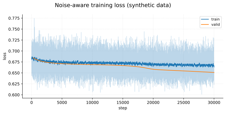
The model is not calibrated at the default decision threshold (0.5) due to imbalance:
t_cal = torch.quantile(trainer.predict_proba(x_train)[:, 1], q=LABEL_PROBS[0])
print(evaluate(trainer, x_train, y_train, t=t_cal)["message"]); print()
print(evaluate(trainer, x_valid, y_valid, t=t_cal)["message"])
[[2320 923]
[ 880 3877]]
m=8000, f1=0.77438, t=0.59114
[[ 533 253]
[ 195 1019]]
m=2000, f1=0.77432, t=0.59114NOTE: Not much better than GenModel. The next sections uses more a realistic dataset.
IMDB Movie Reviews
We apply the same weak supervision pipeline to a real text classification task: IMDB movie review sentiment analysis. The key challenge is adapting our GenModel and NoiseAwareTrainer (designed for tensor inputs) to work with raw text data. We define text-based labeling functions that detect sentiment patterns, wrap them to be tensor-compatible, and use TF-IDF features to train the noise-aware discriminative model.
import re
import pandas as pd
from datasets import load_dataset

RANDOM_SEED = 0
set_seed(RANDOM_SEED)


# Load IMDB dataset (16000 train in total, 1000 valid + 2000 oracle)
ds = load_dataset("imdb")
datasets = {
    "test": ds["test"].shuffle(seed=RANDOM_SEED),
    "train": ds["train"].shuffle(seed=RANDOM_SEED),
}

load_subset = lambda split, n: datasets[split].select(range(*n))
ds_train  = load_subset("train", (0, 16000))
ds_valid  = load_subset("test", (0, 1000))
ds_oracle = load_subset("test", (1000, 3000))

train_texts  = ds_train["text"]
valid_texts  = ds_valid["text"]
oracle_texts = ds_oracle["text"]

train_labels  = torch.tensor(ds_train["label"])   # {0, 1}
valid_labels  = torch.tensor(ds_valid["label"])
oracle_labels = torch.tensor(ds_oracle["label"])

# Slices for training, validation, and oracle sets
y_train, y_valid, y_oracle = {}, {}, {}
x_train, x_valid, x_oracle = {}, {}, {}
L_train, L_valid, L_oracle = {}, {}, {}

# Labeled budget: 400 validation | 200 fine-tuning (disjoint)
y_valid["i=0:400"]   = valid_labels[:400]
y_train["i=0:3000"]  = train_labels[:3000]
y_oracle["i=0:2000"] = oracle_labels[:2000]

K = 2
ABSTAIN = -1
Tip
The convention for the datasets is that train, valid, and oracle are all disjoint corpuses of text and corresponding ground truth labels. Then, we just index on these sets to get specific splits for our experiments. In particular, train has 16,000 data points but we only use a slice of size 3,000 to train the first model, and so on.
Note
In what follows, all training samples are unlabeled. But we reserve a small budget of 400 labeled examples for early stopping and evaluation. Having ground truth is unavoidable. Otherwise, we will make design decisions based on noisy estimates. We will expect that the evals are optimistic since we’re early stopping on the same eval set.
Labeling functions
# (1) Strong adjectives — keyword matching
def lf_strong_sentiment(text):
    text = text.lower()
    pos_words = [
        "excellent", "masterpiece", "outstanding", "brilliant", "perfect",
        "superb", "fantastic", "wonderful", "phenomenal", "magnificent",
        "flawless", "exceptional", "incredible"
    ]
    neg_words = [
        "terrible", "awful", "horrible", "worst", "dreadful", "atrocious",
        "abysmal", "pathetic", "unwatchable", "horrendous", "appalling",
        "garbage", "trash"
    ]
    pos = any(w in text for w in pos_words)
    neg = any(w in text for w in neg_words)
    if pos and not neg: return 1
    if neg and not pos: return 0
    return ABSTAIN


# (2) Balance of positive/negative word counts — keyword counting
def lf_sentiment_words(text):
    text = text.lower()
    pos_words = [
        "great", "love", "amazing", "best", "enjoyed", "favorite", "fun",
        "loved", "beautiful", "impressive", "entertaining", "charming",
        "delightful", "touching", "powerful"
    ]
    neg_words = [
        "bad", "waste", "boring", "poor", "stupid", "annoying", "disappointing",
        "dull", "lame", "mediocre", "pointless", "forgettable", "tedious",
        "ridiculous", "painful"
    ]
    pos_count = sum(1 for w in pos_words if w in text)
    neg_count = sum(1 for w in neg_words if w in text)
    if pos_count > neg_count: return 1
    if neg_count > pos_count: return 0
    return ABSTAIN


# (3) Explicit ratings via regex patterns
def lf_rating_mention(text):
    text = text.lower()
    pos_patterns = [
        r"10/10", r"10 out of 10", r"5 stars", r"5/5", r"9/10",
        r"9 out of 10", r"8/10", r"4/5", r"4 out of 5"
    ]
    neg_patterns = [
        r"1/10", r"1 out of 10", r"1 star[^s]", r"0 stars", r"0/10",
        r"2/10", r"2 out of 10", r"3/10", r"1/5"
    ]
    pos = any(re.search(p, text) for p in pos_patterns)
    neg = any(re.search(p, text) for p in neg_patterns)
    if pos and not neg: return 1
    if neg and not pos: return 0
    return ABSTAIN


# (4) Recommendation / avoidance phrases — keyword matching
def lf_recommendation(text):
    text = text.lower()
    pos_phrases = [
        "highly recommend", "must see", "must watch", "worth watching",
        "go see", "definitely watch", "check it out", "worth every minute",
        "well worth", "do yourself a favor"
    ]
    neg_phrases = [
        "do not recommend", "don't recommend", "avoid", "skip this",
        "don't bother", "don't waste", "stay away", "save your",
        "do not watch", "don't watch this"
    ]
    pos = any(p in text for p in pos_phrases)
    neg = any(p in text for p in neg_phrases)
    if pos and not neg: return 1
    if neg and not pos: return 0
    return ABSTAIN


# (5) Repetition of negative sentiment words (>= 3 distinct) — pile-up heuristic
def lf_neg_pile(text):
    text = text.lower()
    neg_words = [
        "bad", "terrible", "awful", "waste", "boring", "stupid",
        "horrible", "worst", "poor", "disappointing", "dreadful",
        "pathetic", "garbage", "trash", "painful"
    ]
    count = sum(1 for w in neg_words if w in text)
    if count >= 3: return 0
    return ABSTAIN


# (6) Repetition of positive sentiment words (>= 3 distinct) — pile-up heuristic
def lf_pos_pile(text):
    text = text.lower()
    pos_words = [
        "great", "excellent", "amazing", "love", "wonderful",
        "brilliant", "fantastic", "superb", "best", "perfect",
        "beautiful", "incredible", "outstanding"
    ]
    count = sum(1 for w in pos_words if w in text)
    if count >= 3: return 1
    return ABSTAIN


# (7) Profanity / strong negative language — keyword matching
def lf_profanity(text):
    text = text.lower()
    words = [
        "crap", "sucks", "sucked", "crappy", "god-awful", "godawful",
        "piece of shit", "pile of crap", "steaming pile"
    ]
    if any(w in text for w in words):
        return 0
    return ABSTAIN


# (8) Actor/performance praise — keyword matching
def lf_actor_praise(text):
    text = text.lower()
    pos = [
        "brilliant performance", "brilliant acting", "great performance",
        "great acting", "superb acting", "amazing performance", "stellar cast",
        "perfectly cast", "outstanding performance", "wonderful performance",
        "convincing performance", "powerful performance"
    ]
    neg = [
        "terrible acting", "awful performance", "wooden acting",
        "bad acting", "can't act", "overacting", "miscast",
        "worst performance", "laughable acting", "stiff acting"
    ]
    p = any(phrase in text for phrase in pos)
    n = any(phrase in text for phrase in neg)
    if p and not n: return 1
    if n and not p: return 0
    return ABSTAIN


# (9) AFINN-style lexicon scoring — scored word list with threshold
def lf_lexicon_score(text):
    text = text.lower()
    # Manually curated scored words (positive > 0, negative < 0)
    highly_pos  = ["love", "loved", "excellent", "perfect", "amazing", "wonderful", "superb", "outstanding", "fantastic"]
    very_pos    = ["brilliant", "great", "enjoy", "enjoyed", "fun", "beautiful"]
    pos         = ["good", "nice", "fine", "decent"]
    neg         = ["weak", "mediocre", "forgettable", "bland"]
    very_neg    = ["boring", "bad", "waste", "stupid", "poor", "disappointing", "dull", "annoying"]
    highly_neg  = ["hate", "hated", "terrible", "awful", "horrible", "worst"]

    groups = {
         3: highly_pos,  2: very_pos,  1: pos,
        -3: highly_neg, -2: very_neg, -1: neg
    }
    lexicon = {w: s for s, ws in groups.items() for w in ws}
    words = text.split()
    score = sum(lexicon.get(w.strip(".,!?;:\"'()"), 0) for w in words)
    if score >= 5: return 1
    if score <= -5: return 0
    return ABSTAIN


# (10) Negation density — structural/linguistic heuristic
def lf_negation_density(text):
    text = text.lower()
    words = text.split()
    if len(words) < 20: return ABSTAIN
    neg_words = {
        "not", "no", "never", "nothing", "nowhere", "neither",
        "nobody", "don't", "doesn't", "didn't", "won't", "wouldn't",
        "couldn't", "shouldn't", "isn't", "aren't", "wasn't", "weren't",
        "can't", "cannot", "hardly", "barely", "nor"
    }
    neg_count = sum(1 for w in words if w in neg_words)
    density = neg_count / len(words)
    if density > 0.04: return 0  # high negation density -> negative
    return ABSTAIN


# (11) Punctuation-based: exclamation density as emotional intensity proxy
def lf_exclamation_density(text):
    excl_count = text.count("!")
    words = text.split()
    if len(words) < 20: return ABSTAIN
    density = excl_count / len(words)
    if density > 0.03:
        # High exclamation density — check if sentiment words present
        text_lower = text.lower()
        pos = any(w in text_lower for w in ["great", "love", "amazing", "best", "wonderful"])
        neg = any(w in text_lower for w in ["bad", "worst", "terrible", "awful", "hate"])
        if pos and not neg: return 1
        if neg and not pos: return 0
    return ABSTAIN


# (12) Capitalization ratio — structural heuristic (shouting)
def lf_caps_ratio(text):
    words = text.split()
    if len(words) < 20: return ABSTAIN
    caps_words = [w for w in words if w.isupper() and len(w) > 2]
    ratio = len(caps_words) / len(words)
    if ratio < 0.02: return ABSTAIN
    pos = {
        "GREAT", "LOVE", "AMAZING", "BEST", "PERFECT", "AWESOME",
        "WONDERFUL", "BRILLIANT", "FANTASTIC", "EXCELLENT"
    }
    neg = {
        "WORST", "TERRIBLE", "AWFUL", "HORRIBLE", "BAD", "HATE",
        "BORING", "STUPID", "GARBAGE", "TRASH", "WASTE"
    }
    pos_count = sum(1 for w in caps_words if w in pos)
    neg_count = sum(1 for w in caps_words if w in neg)
    if pos_count > neg_count: return 1
    if neg_count > pos_count: return 0
    return ABSTAIN


# (13) Review length heuristic — very long reviews tend positive on IMDB
def lf_length_signal(text):
    words = text.split()
    sentences = [s for s in re.split(r'[.!?]+', text) if s.strip()]
    if len(words) > 400 and len(sentences) > 15:
        return 1  # Long, detailed reviews skew positive
    return ABSTAIN


# (14) Sentence-level sentiment consistency — structural heuristic
def lf_sentence_sentiment(text):
    sentences = [s.strip() for s in re.split(r'[.!?]+', text) if len(s.strip()) > 10]
    if len(sentences) < 3: return ABSTAIN
    pos_words = [
        "great", "love", "amazing", "best", "enjoyed", "wonderful",
        "excellent", "brilliant", "fantastic", "perfect", "beautiful"
    ]
    neg_words = [
        "bad", "terrible", "awful", "boring", "worst", "dull",
        "horrible", "waste", "stupid", "disappointing", "poor"
    ]
    pos_sents = sum(1 for s in sentences if any(w in s.lower() for w in pos_words))
    neg_sents = sum(1 for s in sentences if any(w in s.lower() for w in neg_words))
    total = len(sentences)
    if pos_sents / total > 0.4 and neg_sents / total < 0.1: return 1
    if neg_sents / total > 0.4 and pos_sents / total < 0.1: return 0
    return ABSTAIN


# (15) First/last sentence heuristic — people often state verdict at start/end
def lf_bookend_sentiment(text):
    sentences = [s.strip() for s in re.split(r'[.!?]+', text) if len(s.strip()) > 5]
    if len(sentences) < 3: return ABSTAIN
    bookends = (sentences[0] + " " + sentences[-1]).lower()
    pos = [
        "great", "excellent", "love", "amazing", "wonderful",
        "highly recommend", "fantastic", "must see", "brilliant"
    ]
    neg = [
        "terrible", "awful", "worst", "horrible", "waste",
        "avoid", "boring", "don't bother", "garbage"
    ]
    p = any(w in bookends for w in pos)
    n = any(w in bookends for w in neg)
    if p and not n: return 1
    if n and not p: return 0
    return ABSTAIN


# (16) Comparative structure via regex
def lf_comparative_regex(text):
    text_lower = text.lower()
    # "one of the best/worst X" pattern
    if re.search(r"one of the (best|greatest|finest|most entertaining)", text_lower):
        return 1
    if re.search(r"one of the (worst|most boring|most terrible|most disappointing)", text_lower):
        return 0
    # "the best/worst X i've (ever) seen"
    if re.search(r"the (best|greatest|most amazing).{0,20}(i'?ve|i have).{0,5}(ever )?(seen|watched)", text_lower):
        return 1
    if re.search(r"the (worst|most boring|most awful).{0,20}(i'?ve|i have).{0,5}(ever )?(seen|watched)", text_lower):
        return 0
    return ABSTAIN


# (17) Question density — reviews with many questions tend to be critical
def lf_question_density(text):
    words = text.split()
    if len(words) < 30: return ABSTAIN
    q_count = text.count("?")
    density = q_count / len(words)
    if density > 0.02:  # lots of rhetorical questions -> likely negative
        return 0
    return ABSTAIN


# (18) Contrastive "but" pattern — keyword + structure
def lf_contrastive_but(text):
    text_lower = text.lower()
    # "X but Y" where final clause determines sentiment
    parts = text_lower.split(" but ")
    if len(parts) < 2: return ABSTAIN
    last_part = parts[-1][:200]  # look at what comes after last "but"
    pos = ["enjoyed", "great", "good", "worth", "love", "recommend", "brilliant"]
    neg = ["boring", "bad", "disappointing", "waste", "terrible", "awful", "fails"]
    p = any(w in last_part for w in pos)
    n = any(w in last_part for w in neg)
    if p and not n: return 1
    if n and not p: return 0
    return ABSTAIN


# (19) Emotional punctuation — ellipsis and multiple punctuation marks
def lf_emotional_punctuation(text):
    # Multiple exclamation/question combos suggest strong emotion
    strong = len(re.findall(r'[!?]{2,}', text))
    if strong < 2: return ABSTAIN
    text_lower = text.lower()
    pos = any(w in text_lower for w in ["love", "amazing", "great", "best", "awesome"])
    neg = any(w in text_lower for w in ["hate", "worst", "terrible", "awful", "bad"])
    if pos and not neg: return 1
    if neg and not pos: return 0
    return ABSTAIN


# (20) Hedging language — uncertainty/lukewarm expressions suggest negative
def lf_hedging(text):
    text_lower = text.lower()
    hedges = [
        "i guess", "i suppose", "it's okay", "it's ok", "it was okay",
        "it was ok", "nothing special", "could have been better",
        "not terrible but", "not the worst", "seen worse", "seen better",
        "meh", "so-so"
    ]
    if sum(1 for h in hedges if h in text_lower) >= 2:
        return 0  # multiple hedges -> lukewarm/negative
    return ABSTAIN


text_lfs = [
    lf_strong_sentiment,       # 0  keyword matching
    lf_sentiment_words,        # 1  keyword counting
    lf_rating_mention,         # 2  regex patterns
    lf_recommendation,         # 3  keyword matching
    lf_neg_pile,               # 4  pile-up heuristic
    lf_pos_pile,               # 5  pile-up heuristic
    lf_profanity,              # 6  keyword matching
    lf_actor_praise,           # 7  keyword matching
    lf_lexicon_score,          # 8  scored lexicon
    lf_negation_density,       # 9  structural/linguistic
    lf_exclamation_density,    # 10 punctuation + keyword
    lf_caps_ratio,             # 11 capitalization structure
    lf_length_signal,          # 12 length heuristic
    lf_sentence_sentiment,     # 13 sentence-level structure
    lf_bookend_sentiment,      # 14 positional heuristic
    lf_comparative_regex,      # 15 regex patterns
    lf_question_density,       # 16 punctuation structure
    lf_contrastive_but,        # 17 discourse structure
    lf_emotional_punctuation,  # 18 punctuation + keyword
    lf_hedging,                # 19 hedging/uncertainty
]
Peeking into the latent vs estimated performance of the LFs:
Code
# Coverage, accuracy, and F1 on train set
LF_STRATEGIES = {
    "lf_strong_sentiment": "Strong pos/neg keywords",
    "lf_sentiment_words": "Count pos vs neg keywords",
    "lf_rating_mention": "Regex: explicit ratings (e.g. \"8/10\")",
    "lf_recommendation": "Keywords: \"recommend\", \"must see\", etc.",
    "lf_neg_pile": "Pile-up: ≥3 neg words in sentence",
    "lf_pos_pile": "Pile-up: ≥3 pos words in sentence",
    "lf_profanity": "Profanity keywords ↦ negative",
    "lf_actor_praise": "Keywords: actor/director praise",
    "lf_lexicon_score": "Scored lexicon: Σ(word scores) ≷ ±𝜏",
    "lf_negation_density": "Structural: #negations / #words",
    "lf_exclamation_density": "Exclamation marks + pos/neg context",
    "lf_caps_ratio": "ALL-CAPS sentiment words ratio",
    "lf_length_signal": "Review length (very long ↦ pos)",
    "lf_sentence_sentiment": "Sentence-level sentiment consistency",
    "lf_bookend_sentiment": "Opening + closing sentence polarity",
    "lf_comparative_regex": "Regex: \"one of the best/worst\" patterns",
    "lf_question_density": "High question ratio ↦ negative",
    "lf_contrastive_but": "\"but\" clause polarity (final clause wins)",
    "lf_emotional_punctuation": "\"!!!\" / \"...\" patterns",
    "lf_hedging": "(\"seen worse\", \"so-so\") ↦ neg",
}

stats = []
for lf in text_lfs:
    outputs = [lf(t) for t in train_texts]
    labels = train_labels.numpy()
    fired = [i for i, o in enumerate(outputs) if o != ABSTAIN]
    cov = len(fired) / len(outputs)
    actual_f1 = f1_score([labels[i] for i in fired], [outputs[i] for i in fired], average="weighted") if fired else 0.0

    valid_outputs = [lf(t) for t in valid_texts[:400]]
    valid_fired = [i for i, o in enumerate(valid_outputs) if o != ABSTAIN]
    valid_cov = len(valid_fired) / len(valid_outputs)
    valid_f1 = f1_score([y_valid["i=0:400"][i] for i in valid_fired], [valid_outputs[i] for i in valid_fired], average="weighted") if valid_fired else 0.0

    stats.append({
        "LF": lf.__name__,
        "Strategy": LF_STRATEGIES.get(lf.__name__, ""),
        "cov (%)": f"{cov * 100:.1f}",
        "cov (valid)": f"{valid_cov * 100:.1f}",
        "F1": f"{actual_f1:.3f}",
        "F1 (valid)": f"{valid_f1:.3f}",
    })

pd.DataFrame(stats)| LF | Strategy | cov (%) | cov (valid) | F1 | F1 (valid) | |
|---|---|---|---|---|---|---|
| 0 | lf_strong_sentiment | Strong pos/neg keywords | 43.8 | 45.5 | 0.862 | 0.835 |
| 1 | lf_sentiment_words | Count pos vs neg keywords | 74.7 | 74.5 | 0.774 | 0.761 |
| 2 | lf_rating_mention | Regex: explicit ratings (e.g. "8/10") | 5.2 | 5.5 | 0.915 | 0.954 |
| 3 | lf_recommendation | Keywords: "recommend", "must see", etc. | 13.3 | 9.8 | 0.807 | 0.897 |
| 4 | lf_neg_pile | Pile-up: ≥3 neg words in sentence | 10.4 | 10.0 | 0.911 | 1.000 |
| 5 | lf_pos_pile | Pile-up: ≥3 pos words in sentence | 15.1 | 13.5 | 0.762 | 0.630 |
| 6 | lf_profanity | Profanity keywords ↦ negative | 6.5 | 6.5 | 0.757 | 0.943 |
| 7 | lf_actor_praise | Keywords: actor/director praise | 5.3 | 6.8 | 0.863 | 0.886 |
| 8 | lf_lexicon_score | Scored lexicon: Σ(word scores) ≷ ±𝜏 | 36.5 | 37.0 | 0.880 | 0.855 |
| 9 | lf_negation_density | Structural: #negations / #words | 3.2 | 4.5 | 0.662 | 0.533 |
| 10 | lf_exclamation_density | Exclamation marks + pos/neg context | 2.3 | 2.5 | 0.882 | 0.691 |
| 11 | lf_caps_ratio | ALL-CAPS sentiment words ratio | 0.9 | 1.8 | 0.797 | 1.000 |
| 12 | lf_length_signal | Review length (very long ↦ pos) | 12.5 | 8.2 | 0.371 | 0.284 |
| 13 | lf_sentence_sentiment | Sentence-level sentiment consistency | 6.1 | 6.0 | 0.966 | 1.000 |
| 14 | lf_bookend_sentiment | Opening + closing sentence polarity | 27.4 | 29.0 | 0.820 | 0.833 |
| 15 | lf_comparative_regex | Regex: "one of the best/worst" patterns | 7.7 | 8.0 | 0.910 | 0.937 |
| 16 | lf_question_density | High question ratio ↦ negative | 2.5 | 3.2 | 0.692 | 0.469 |
| 17 | lf_contrastive_but | "but" clause polarity (final clause wins) | 20.3 | 23.2 | 0.701 | 0.709 |
| 18 | lf_emotional_punctuation | "!!!" / "..." patterns | 1.4 | 1.0 | 0.810 | 0.500 |
| 19 | lf_hedging | ("seen worse", "so-so") ↦ neg | 0.7 | 0.8 | 0.649 | 0.533 |
Tip
Here we see the difference between actual LF quality vs. estimate from the 400 labeled sample that we have. In practice you get to only see the valid columns. That is, you will have to navigate with imperfect information with the difference becoming larger the noisier your dataset is. For example, we will probably reject lf_question_density and lf_emotional_punctuation with valid F1 ≤ 0.5 even if the latent F1=0.692 and 0.810, respectively.
Model training
LF outputs & features. Here we precompute the LF outputs for the raw reviews and stack them into \Lambda matrices, mirroring the above synthetic pipeline. We also extract TF-IDF features as the input representation for the discriminative model:
from sklearn.feature_extraction.text import TfidfVectorizer

def build_L_text(labeling_funcs, texts):
    """Build LF output matrix from text labeling functions."""
    return torch.tensor([[lf(t) for lf in labeling_funcs] for t in texts])

# LF matrices (independent of feature variant)
L_valid["i=0:400"]    = build_L_text(text_lfs, valid_texts[:400])
L_train["i=0:3000"]   = build_L_text(text_lfs, train_texts[:3000])
L_oracle["i=0:2000"]  = build_L_text(text_lfs, oracle_texts[:2000])

# 5k unigram TF-IDF features on train set (3000 reviews)
vec_5k = TfidfVectorizer(max_features=5000)
vec_5k.fit(train_texts[:3000])

f_vec = lambda vec, texts: torch.tensor(vec.transform(texts).toarray(), dtype=torch.float32)
x_valid["i=0:400,d=5k"]     = f_vec(vec_5k, valid_texts[:400])
x_train["i=0:3000,d=5k"]    = f_vec(vec_5k, train_texts[:3000])
x_oracle["i=0:2000,d=5k"]   = f_vec(vec_5k, oracle_texts[:2000])
Generative model. We train GenModel on the text LF outputs with a balanced prior. The model learns the latent confusion matrix of each LF and produces soft labels p_{\hat{\Phi}}(y \mid \lambda_{\textbf{\textsf{x}}_i}) for every review:
IMDB_LABEL_PROBS = {0: 0.50, 1: 0.50}

# can use L_valid to validate since there's no early stopping leakage
gen_model_imdb = GenModel(num_classes=2, num_lfs=len(text_lfs), class_prior=IMDB_LABEL_PROBS)
history_gen_imdb = gen_model_imdb.fit(L_train["i=0:3000"], L_valid["i=0:400"], epochs=1000, lr=0.03)
Tip
The prior labels IMDB_LABEL_PROBS can also be estimated from the curated validation set.
Training and validation NLL for the generative model:
Code
plt.figure(figsize=(5, 3))
plt.plot(history_gen_imdb["train"], label="train")
plt.plot(history_gen_imdb["valid_steps"], history_gen_imdb["valid"], label="valid")
plt.legend()
plt.xlabel("step")
plt.ylabel("NLL")
plt.grid(linestyle="dotted", alpha=0.6);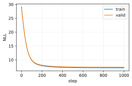
Noise-aware training. We train an MLP on TF-IDF features using the noise-aware loss, weighted by the generative model’s soft labels. The discriminative model can generalize beyond the keywords used in the LFs by leveraging the full TF-IDF vocabulary:
set_seed(RANDOM_SEED)

clf_imdb = nn.Sequential(
    nn.Linear(5000, 32),
    nn.SELU(),
    nn.Linear(32, K)
)

trainer_imdb = NoiseAwareTrainer(clf_imdb, gen_model_imdb)
history_imdb = trainer_imdb.fit(
    x_train["i=0:3000,d=5k"], L_train["i=0:3000"], x_valid["i=0:400,d=5k"], y_valid["i=0:400"],
    epochs=300, bs=64, lr=0.003, alpha=0.0, momentum=0.9,
)
seed: 0 deterministic: FalseEarly stopping at epoch 119...
Training stopped.
Best train loss: 0.2931 | Best valid loss: 0.4076Training and validation loss for the noise-aware discriminative model:
plot_history(history_imdb, title="Noise-aware training loss (IMDB)")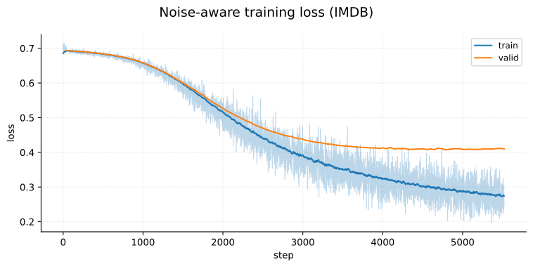
Evaluation
print("GenModel (IMDB):")
print(evaluate(gen_model_imdb, L_train["i=0:3000"], y_train["i=0:3000"])["message"]); print()
print(evaluate(gen_model_imdb, L_valid["i=0:400"],  y_valid["i=0:400"])["message"])

print("\nNoiseAwareTrainer (IMDB):")
print(evaluate(trainer_imdb, x_train["i=0:3000,d=5k"], y_train["i=0:3000"])["message"]); print()
print(evaluate(trainer_imdb, x_valid["i=0:400,d=5k"],  y_valid["i=0:400"])["message"])
GenModel (IMDB):
[[1187 321]
[ 286 1206]]
m=3000, f1=0.79765, t=0.50000
[[150 48]
[ 39 163]]
m=400, f1=0.78234, t=0.50000
NoiseAwareTrainer (IMDB):
[[1219 289]
[ 268 1224]]
m=3000, f1=0.81433, t=0.50000
[[159 39]
[ 32 170]]
m=400, f1=0.82241, t=0.50000Unlike in the toy dataset, the NAT model outperforms GenModel on IMDB reviews. While the generative model can only make predictions from “finite” LF output patterns, the discriminative model leverages TF-IDF feature vectors to capture sentiment signals beyond the heuristics hardcoded in the LFs. This turns out to matter for a real dataset.
Self-training on pseudo-labels
Recall that we have the following pipeline for the generative model G:
{\textbf{\textsf{x}}} \underset{\Lambda}{\mapsto} \lambda_{\textbf{\textsf{x}}} \underset{G}{\mapsto} p(\cdot \mid \lambda_\textsf{x}) \in [0, 1]^K.
This is what we use to supervise the NAT model f_{\text{NAT}}. However, once training is done, the resulting model operates on the inputs without requiring information from the LFs. This is the core advantage of the NAT model: it modulates on complex learned features and representations which can assign confident predictions on examples where labeling functions abstain or disagree on — precisely the data points where the generative model’s signal is weakest.
Self-training exploits this: we take the trained NAT model (the “base model”), use its confident predictions on an unlabeled pool as pseudo-labels, and retrain (i.e. the same architecture) on the original generative model targets + these self-generated pseudo-labels. This explains why its called “self-training”. Note warm-starting from the base weights hurt performance in our experiments. One possible explanation is that the pseudo-label loss provides useful gradient signal precisely when the posterior estimates are noisy, and random initialization gives the optimizer more freedom to find a better basin; starting from NAT weights may bias the search toward a region that is well-calibrated for the NAT loss but suboptimal for the augmented objective.
Augmented dataset. Let f_{\text{NAT}} be the base model and we have the posterior from the generative model. We construct the augmented training set by constructing two datasets defined as follows and taking their union:
\begin{aligned} \mathcal{D}_{\text{gen}} &= \bigl\{\bigl(\textbf{\textsf{x}}_i,\, \tilde{\textbf{\textsf{p}}}_i = p_{\hat{\Phi}}(y \mid \lambda_{\textbf{\textsf{x}}_i})\bigr)\bigr\}_{i=1}^{M}, \\ \mathcal{D}_{\text{pseudo}} &= \bigl\{\bigl(\textbf{\textsf{x}}_i,\, \tilde{\textbf{\textsf{p}}}_i = \text{Softmax}(f_{\text{NAT}}(\textbf{\textsf{x}}_i))\bigr) : \textbf{\textsf{x}}_i \in \mathcal{U},\, w_i \geq \tau_{\text{conf}}\bigr\}, \end{aligned}
where \mathcal{U} is the unlabeled pool, w_i = \max_k\, \tilde{p}_{ik} is the base model’s confidence, and \tau_{\text{conf}} is a threshold (0.85 in our experiments). The second coordinate in each pair is a soft label \tilde{\textbf{\textsf{p}}}_i \in \Delta^{K-1} — a probability vector over the K classes rather than a hard one-hot label, where \Delta^{K-1} = \{\textbf{\textsf{q}} \in \mathbb{R}^K : q_k \ge 0,\, \sum_k q_k = 1\} is the (K{-}1)-dimensional probability simplex. The self-trained model is trained on \mathcal{D} = \mathcal{D}_{\text{gen}} \cup \mathcal{D}_{\text{pseudo}} with confidence-weighted soft cross-entropy, where each example is weighted by its confidence w_i = \max_k\, \tilde{p}_{ik}:
\begin{aligned} \mathcal{L}_{\text{self}}(\Theta) &= -\frac{1}{B} \sum_{i \in \mathcal{B}} w_i \sum_{k=0}^{K-1} \tilde{p}_{ik}\, \log \hat{p}_{\Theta,ik} \\ &= -\frac{1}{B_{\text{gen}} + B_{\text{pseudo}}} \sum_{i \in \mathcal{B}_{\text{gen}}} w_i \sum_{y=0}^{K-1} {p_{\hat{\Phi}}(y \mid \lambda_{\textbf{\textsf{x}}_i})} \, \log \hat{p}_{\Theta,iy} \\ &+ -\frac{1}{B_{\text{gen}} + B_{\text{pseudo}}} \sum_{i \in \mathcal{B}_{\text{pseudo}}} w_i \sum_{k=0}^{K-1} \tilde{p}_{ik}^{\text{NAT}} \, \log \hat{p}_{\Theta,ik}, \end{aligned}
where \hat{\textbf{\textsf{p}}}_{\Theta,i} = \text{Softmax}(f_\Theta(\textbf{\textsf{x}}_i)) is the self-trained model’s predicted distribution and \mathcal{B} = \mathcal{B}_{\text{gen}} \cup \mathcal{B}_{\text{pseudo}} is a mini-batch drawn from \mathcal{D}.
Tip
\mathcal{L}_{\text{self}} is the original NAT loss augmented with the pseudo-label loss on the unlabeled pool \mathcal{U}. That is, self-training simply extends NAT training to include confident predictions from the base model on an unlabeled pool as additional supervision.
Note
On soft labels. We initially tried hard pseudo-labels via argmax. But this didn’t turn out to be consistent over upstream hyperparameter choices (e.g. its too sensitive to the GenModel). This makes sense since labels via argmax are lossy: small shifts in the generative model’s convergence can flip labels near the decision boundary, cascading errors into the self-trained model. (1) Soft targets preserve the label model’s uncertainty, and (2) confidence weighting ensures that examples where the generative model or base model is unsure contribute proportionally less to the gradient. This makes the pipeline more robust to hyperparameter choices upstream.
Why use the generative model posterior along with \mathcal{D}_{\text{pseudo}}? In NAT training, the generative model posterior steers the loss because the true label is unknown and the model has no prior knowledge of \textbf{\textsf{x}} — every candidate label must contribute, weighted by LF-derived confidence. But by self-training time, the base model has learned a feature-based mapping: its confident outputs already encode the relationship between \textbf{\textsf{x}} and y, making them strictly more informative than the generative model’s feature-blind posterior. We use these as \mathcal{D}_{\text{pseudo}}.
However, the base model is only confident on a filtered subset of the pool (w_i \geq \tau_{\text{conf}}), so coverage is incomplete. \mathcal{D}_{\text{gen}} fills this gap: on the original training set where LFs fire, the confidence weighted generative model posterior is still the best available signal and anchors the self-trained model on the LF-covered region. During SGD, mini-batches are drawn from \mathcal{D} = \mathcal{D}_{\text{gen}} \cup \mathcal{D}_{\text{pseudo}}, so the mixing ratio (|\mathcal{D}_{\text{gen}}| : |\mathcal{D}_{\text{pseudo}}| \approx 3:2 in our experiments) controls how much each supervision signal contributes to the gradient on average.
Base model
Since this requires a stronger base model, we expand the NAT training set from 3000 to 6000 reviews and switch to bigram TF-IDF (ngram_range=(1, 2), 7000 features), which captures multi-word phrases like “waste of time” or “must watch” that unigram TF-IDF misses. The original generative model (trained on 3000 reviews) is reused to produce soft labels for all 6000 points4. We keep the same validation set throughout to ensure comparisons are valid.
set_seed(RANDOM_SEED)

# Larger training set: 6000 reviews
y_train["i=0:6000"] = train_labels[:6000]
L_train["i=0:6000"] = build_L_text(text_lfs, train_texts[:6000])

# Reuse the original generative model — retraining on 6k hurts performance
# Bigram TF-IDF with 7k features w/ sublinear scaling of TF: i.e. 1 + log(TF)
vec_7k = TfidfVectorizer(max_features=7000, ngram_range=(1, 2), sublinear_tf=True)
vec_7k.fit(train_texts[:6000])

x_valid["i=0:400,d=7k"]     = f_vec(vec_7k, valid_texts[:400])
x_train["i=0:6000,d=7k"]    = f_vec(vec_7k, train_texts[:6000])
x_oracle["i=0:2000,d=7k"]   = f_vec(vec_7k, oracle_texts[:2000])
Model. The baseline MLP uses a single hidden layer of 32 units which bottlenecks the 5000 input features. We widen the base model to two hidden layers (128 and 32 units) and add L2 regularization (weight_decay=1e-4) to prevent overfitting on noisy soft labels:
set_seed(RANDOM_SEED)

def make_clf_v2():
    return nn.Sequential(
        nn.Linear(7000, 128), nn.SELU(),
        nn.Linear(128, 32), nn.SELU(),
        nn.Linear(32, K),
    )

1trainer_v2 = NoiseAwareTrainer(make_clf_v2(), gen_model_imdb)
history_v2 = trainer_v2.fit(
    x_train["i=0:6000,d=7k"], L_train["i=0:6000"],
    x_valid["i=0:400,d=7k"], y_valid["i=0:400"],
    epochs=300, bs=64, lr=0.003, alpha=1e-4, momentum=0.9,
)

print()
print("NAT v2 (IMDB, valid):")
print(evaluate(trainer_v2, x_valid["i=0:400,d=7k"], y_valid["i=0:400"])["message"])- 1
- The original generative model (trained on 3k) is reused as-is. Its confusion matrices already capture the LF statistics well; applying them to the 6k training set requires only forward inference.
seed: 0 deterministic: FalseEarly stopping at epoch 35...
Training stopped.
Best train loss: 0.3214 | Best valid loss: 0.4021
NAT v2 (IMDB, valid):
[[165 33]
[ 32 170]]
m=400, f1=0.83749, t=0.50000
Note
NAT v2 achieves F1 = 0.8324 — a +2.0pp improvement over the baseline (0.8125). The richer features and more data significantly improved performance. Further payoff comes in the next step. For instance, NAT v2 produces more pseudo-labeled examples than the baseline NAT at higher oracle accuracy.
Pseudo-labeling. We apply NAT v2 to 10,000 held-out reviews (indices 6000–16000, disjoint from training and validation) and retain predictions with \max_y\, p(y \mid \textbf{\textsf{x}}) \geq 0.85 as pseudo-labels. We also record oracle accuracy — the fraction of pseudo-labels that match the true IMDB labels — as a proxy for pseudo-label quality:
set_seed(RANDOM_SEED)

# Unlabeled pool: 10k reviews disjoint from train/valid
y_train["i=6000:16000"]         = train_labels[6000:16000]
x_train["i=6000:16000,d=7k"]    = f_vec(vec_7k, train_texts[6000:16000])
y_pool = y_train["i=6000:16000"]
x_pool = x_train["i=6000:16000,d=7k"]

# Get confident pseudo-labels
p_pool = trainer_v2.predict_proba(x_pool)  # (10000, 2)
confidence_v2, pseudo_labels = p_pool.max(dim=1)

CONF_THRESHOLD = 0.85
mask_v2 = confidence_v2 >= CONF_THRESHOLD
n_conf = mask_v2.sum().item()
pseudo_acc = (pseudo_labels[mask_v2] == y_pool[mask_v2]).float().mean()

print(f"Confident predictions: {n_conf}/{len(mask_v2)} ({n_conf/len(mask_v2):.1%})")
print(f"Pseudo-label accuracy (oracle check): {pseudo_acc:.3f}")
seed: 0 deterministic: False
Confident predictions: 4759/10000 (47.6%)
Pseudo-label accuracy (oracle check): 0.959NAT v2 labels 47.6% of the pool at 95.9% oracle accuracy. As an exercise, you can show that the baseline NAT labels 45.2% at 95.4% accuracy. The stronger base model produces ~250 more pseudo-labeled examples at a slightly higher per-sample accuracy.
Self-trained model
Combined generative and pseudo-labeled targets to train the self-trained model:
np.random.seed(RANDOM_SEED)
torch.manual_seed(RANDOM_SEED)

# Soft labels from generative model for original training set
p_gen = gen_model_imdb.predict_proba(L_train["i=0:6000"])

# Soft pseudo-labels from NAT base model, filtered by confidence
x_pool = x_train["i=6000:16000,d=7k"]
p_pool = trainer_v2.predict_proba(x_pool)
x_combined = torch.cat([x_train["i=0:6000,d=7k"], x_pool[mask_v2]], dim=0)
targets_combined = torch.cat([p_gen, p_pool[mask_v2]], dim=0)

print(f"Combined training set: {x_combined.shape[0]} examples")
print(f"  Soft labels from gen model: {x_train["i=0:6000,d=7k"].shape[0]}")
print(f"  Pseudo-labeled (confident): {mask_v2.sum().item()}")
Combined training set: 10759 examples
Soft labels from gen model: 6000
Pseudo-labeled (confident): 4759The full pipeline is encapsulated in PseudoLabelSelfTrainer. Given a generative model and a trained base model (NAT). It (1) obtains posterior probability distributions from the generative model posterior, (2) scores an unlabeled pool with the base model and retains confident predictions where w_i = \max \hat{p}_i \geq \tau_{\text{conf}}, and (3) trains on the combined dataset using soft cross-entropy, weighting each example by its confidence w_i:
class PseudoLabelSelfTrainer(Predictor):
    def __init__(self, clf, gen_model, trainer: NoiseAwareTrainer, conf_threshold=0.85):
        super().__init__(clf, gen_model.K, output_probs=False)
        self.clf = clf
        self.trainer = trainer
        self.gen_model = gen_model
        self.conf_threshold = conf_threshold

    def __call__(self, x):
        return self.clf(x)

    def build_pseudo_labels(self, x_pool):
        with torch.inference_mode():
            probs = self.trainer.predict_proba(x_pool)
            mask = probs.max(dim=1).values >= self.conf_threshold
            return mask, probs

    def build_gen_labels(self, L):
        return self.gen_model.predict_proba(L)

    def build_train_dataset(self, x_train, x_pool, L_train):
        p_gen = self.build_gen_labels(L_train)                              # (M, K) gen probas
        mask, p_pseudo = self.build_pseudo_labels(x_pool)                   # filter + nat probas
        x_combined = torch.cat([x_train, x_pool[mask]], dim=0)
        p_combined = torch.cat([p_gen, p_pseudo[mask]], dim=0)
        weights = p_combined.max(dim=1).values                              # confidence weights
        return x_combined, p_combined, weights

    def fit(self, x_train, x_pool, L_train, x_valid, y_valid, epochs=10, bs=8, lr=0.001, alpha=0.0, momentum=0.1, optimizer="sgd"):
        x_combined, p_combined, weights = self.build_train_dataset(x_train, x_pool, L_train)
        return train_cross_entropy(
            self.clf,
            x_combined, p_combined,
            x_valid, y_valid,
            weights=weights,
            epochs=epochs, bs=bs, lr=lr, alpha=alpha, momentum=momentum,
            optimizer=optimizer
        )
Recall F.cross_entropy supports soft targets in the targets argument.
set_seed(RANDOM_SEED)

self_trainer = PseudoLabelSelfTrainer(make_clf_v2(), gen_model_imdb, trainer_v2, conf_threshold=CONF_THRESHOLD)
self_history = self_trainer.fit(
    x_train["i=0:6000,d=7k"],
    x_pool=x_train["i=6000:16000,d=7k"],
    L_train=L_train["i=0:6000"],
    x_valid=x_valid["i=0:400,d=7k"], y_valid=y_valid["i=0:400"],
    epochs=300, bs=64, lr=0.003, alpha=1e-4, momentum=0.9
)
seed: 0 deterministic: FalseEarly stopping at epoch 25...
Training stopped.
Best train loss: 0.2634 | Best valid loss: 0.3925print("Self-trained model (valid):")
print(evaluate(self_trainer, x_valid["i=0:400,d=7k"], y_valid["i=0:400"])["message"])Self-trained model (valid):
[[160 38]
[ 27 175]]
m=400, f1=0.83733, t=0.50000plot_history(self_history, title="Self-training loss (6000 posterior + pseudo)")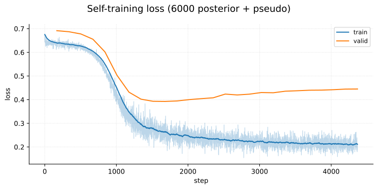
Figure. Recall that our validation loss is always different from the training loss (starting from NAT). Here the train loss is one magnitude lower which is expected since it’s scaled by weights w \in [0, 1].
Supervised fine-tuning
We reserve a separate set of 200 labeled examples (disjoint from the 400 used for evaluation) to fine-tune the self-trained model. We run a few additional epochs of standard cross-entropy on top of self_trainer.clf — the weights are already well-initialized from self-training, so even a small labeled signal can correct residual errors near the decision boundary:
import copy

set_seed(RANDOM_SEED)
1clf_ft = copy.deepcopy(self_trainer.clf)
y_valid["i=400:600"] = valid_labels[400:600]
x_valid["i=400:600,d=7k"] = f_vec(vec_7k, valid_texts[400:600])

history_ft = train_cross_entropy(
    clf_ft,
2    x_train=x_valid["i=400:600,d=7k"],
    y_train=y_valid["i=400:600"],
    x_valid=x_valid["i=0:400,d=7k"],
    y_valid=y_valid["i=0:400"],
3    epochs=300, bs=32, lr=0.0003, alpha=1e-5, momentum=0.9
)

predictor_ft = Predictor(clf_ft, K)
print("Fine-tuned model (valid):")
print(evaluate(predictor_ft, x_valid["i=0:400,d=7k"], y_valid["i=0:400"], t=0.5)["message"])- 1
-
Fine-tuning from
self_trainer.clfweights rather than random initialization is critical: the model already understands the task, so the 200 labels only need to nudge the decision boundary, not learn representations from scratch. - 2
-
Fine-tune on a separate 200 labeled examples (
x_valid["i=400:600,d=7k"]), disjoint from the 400 used for validation. - 3
- Since this is fine-tuning on hard labels, we set a small LR (i.e. 10x smaller compared to NAT / self-training). Since we decreased LR, we decrease B from 64 -> 32.
seed: 0 deterministic: FalseEarly stopping at epoch 175...
Training stopped.
Best train loss: 0.0659 | Best valid loss: 0.3666
Fine-tuned model (valid):
[[163 35]
[ 25 177]]
m=400, f1=0.84987, t=0.50000plot_history(history_ft, title="Fine-tuning loss (200 labeled examples)")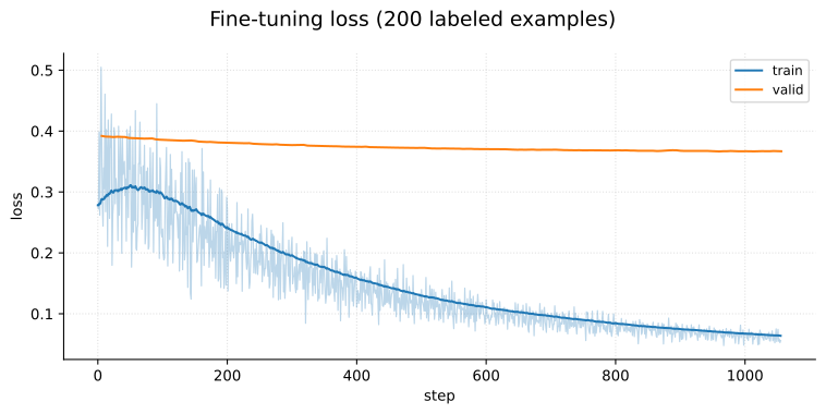
Self-Training with Attention
The approach below is adapted from ASTRA (Karamanolakis et al. 2021) (Automated Self-Training with Rule Attention), which introduces the idea of an attention-based teacher that treats labeling functions and the student as voters. We adapt this core idea to our generative model pipeline with a simplified attention mechanism. The two limitations of vanilla self-training that motivate this extension are:
Fixed aggregation. In self-training, the soft labels come from two fixed sources — the generative model (which weights all LFs equally via confusion matrices) and the NAT teacher (which ignores LFs entirely). Neither adapts which LFs to trust based on the specific input. For instance,
lf_rating_mentionis highly reliable when a review contains “10/10” but misleading when the pattern appears quoted in a negative review5 — the generative model cannot make this distinction.No feedback loop. The self-training student’s predictions are never fed back to improve the label aggregation. If the student learns useful structure beyond what the LFs capture, that knowledge is wasted — it cannot help the system decide which LFs to trust on ambiguous instances.
To address these, we replace both fixed sources with a learned teacher network that produces soft labels \tilde{\textbf{\textsf{p}}}_i by attending over J + 1 voters: the J labeling functions plus the current student’s own prediction. The teacher is supervised on a small labeled set, learning when each LF (and the student) is reliable for a given input. Since the teacher consumes student predictions and the student learns from teacher soft-labels, the two networks undergo co-evolution, yielding progressively better training labels over multiple rounds.
Student network
The student is a small MLP f_\Theta\colon \mathbb{R}^p \to \mathbb{R}^K with the same architecture as the NAT discriminative model — two hidden SELU layers. Because the randomly initialized teacher relies on student outputs, the student is warm-started with NAT weights to avoid degenerate feedback loops in early rounds. Then, the student is further trained each round on the teacher’s aggregated soft labels using a confidence-weighted cross-entropy loss:
\mathcal{L}_{S}(\Theta) = -\frac{1}{M}\sum_{i=1}^M w_i \sum_{k=0}^{K-1} \tilde{p}_{ik} \log \hat{p}_{\Theta,ik}, \quad w_i = \max_k \tilde{p}_{ik},
where \hat{\textbf{\textsf{p}}}_{\Theta,i} = \text{Softmax}(f_\Theta(\textbf{\textsf{x}}_i)) \in \Delta^{K-1} is the student’s predicted distribution, \tilde{\textbf{\textsf{p}}}_i \in \Delta^{K-1} is the soft label produced by the teacher (defined shortly below), and \Delta^{K-1} = \{\textbf{\textsf{q}} \in \mathbb{R}^K : q_k \ge 0,\, \sum_k q_k = 1\} is the probability simplex.
NAT_V2_STATE = copy.deepcopy(trainer_v2.clf.state_dict())   # warm-start reference

def make_student(state_dict=None):
    clf = make_clf_v2()
    if state_dict is not None:
        clf.load_state_dict(copy.deepcopy(state_dict))
    return clf
Teacher network
The teacher network consists of a query encoder followed by an attention mechanism that follows the standard query-key-value pattern. The LFs and students correspond to keys that are dotted with the query vector of the current instance. Then the output probability vector \tilde{\textbf{\textsf{p}}} is calculated by using the attention probabilities as weights for the LF and student vote value vectors.
More precisely, the teacher network consists of the ff. elements:
Query encoder. For each instance \textbf{\textsf{x}} \in \mathbb{R}^p we first compute a query vector:
\textbf{\textsf{q}} = \text{SELU}(\mathbf{W}_q\, \textbf{\textsf{x}}) \in \mathbb{R}^d, where \mathbf{W}_q \in \mathbb{R}^{d \times p} is a learned projection (d = 64 in our implementation). Intuitively, \textbf{\textsf{q}} captures which features of the input are most relevant for deciding which voters to trust — analogous to the query in standard attention that determines what to retrieve.Keys (voter scoring). There are J + 1 voters: the J labeling functions plus the student’s own soft prediction. A linear layer projects the query into a score for each voter — effectively, each row of \mathbf{W}_k acts as a learned key embedding for voter j:
\textbf{\textsf{s}} = \mathbf{W}_k\, \textbf{\textsf{q}} \in \mathbb{R}^{J+1}, \quad \mathbf{W}_k \in \mathbb{R}^{(J+1) \times d}. Each score s_{j} measures how well voter j’s implicit key matches the query instance.Masked-softmax attention. An LF that abstains on \textbf{\textsf{x}} should receive zero weight. We define a mask vector \textbf{\textsf{m}} \in \{0, -\infty\}^{J+1} where m_{j} = -\infty if voter j abstains and 0 otherwise (the student never abstains). The attention weights are then:
\boldsymbol{\alpha} = \text{Softmax}\left(\frac{\textbf{\textsf{s}} + \textbf{\textsf{m}}}{\tau}\right). The -\infty entries exponentiate to zero, ensuring abstaining voters are excluded from the weighted sum. This incorporates a temperature parameter \tau > 0. We set the default value \tau = 0.7 to slightly sharpen the attention.Values (voter labels). Each non-abstaining LF voter j \le J contributes a value — a one-hot label vector \textbf{\textsf{v}}^j = \textbf{\textsf{e}}_{\lambda_j(\textbf{\textsf{x}})} \in \{0,1\}^K. The student contributes its current soft prediction \textbf{\textsf{v}}^{J+1} = \hat{\textbf{\textsf{p}}}_{\Theta} \in \Delta^{K-1}. Note that unlike standard attention where values are learned embeddings, here the values are fixed label vectors determined by each voter’s output.
Aggregated soft label. The teacher output is the attention-weighted sum of voter values — the standard attention readout:
\tilde{\textbf{\textsf{p}}}_i = \sum_{j=1}^{J+1} \alpha_{j}\, \textbf{\textsf{v}}^{j} \in \Delta^{K-1}.
NOTE: If every LF abstains on \textbf{\textsf{x}}, then there is no LF signal to attend over. In that case we fall back to the generative model posterior: \tilde{\textbf{\textsf{p}}} = p_{\hat\Phi}(y \mid \lambda_{\textbf{\textsf{x}}}) (roughly the supplied label prior). This makes sense, otherwise the student will be trained on its own outputs for precisely those examples that are signaled as hard by the LFs. In fact, removing the fallback makes the student train very slowly from our tests. It follows that GenModel posterior probs and the student probs have to be supplied for each input:
class RuleAttentionTeacher(nn.Module):
    def __init__(self, n_features, n_classes, n_lfs, hidden_dim=64, temperature=0.7):
        super().__init__()
        self.query_encoder = nn.Sequential(nn.Linear(n_features, hidden_dim), nn.SELU())
        self.n_lfs = n_lfs
        self.n_classes = n_classes
        self.temperature = temperature
        self.key_proj = nn.Linear(hidden_dim, n_lfs + 1)

    def forward(self, x, L, gen_probs, student_probs):
        B, J, K = x.shape[0], self.n_lfs, self.n_classes
        scores = self.key_proj(self.query_encoder(x)).clone()

        abstain = (L == -1).to(torch.bool)
        lf_mask = torch.zeros(B, J, device=x.device).masked_fill(abstain, float("-inf"))
        mask = torch.cat([lf_mask, torch.zeros(B, 1, device=x.device)], dim=1)
        attn_weights = torch.softmax((scores + mask) / self.temperature, dim=1)

        values = F.one_hot(L.masked_fill(abstain, 0), num_classes=K).to(torch.float32)
        values = torch.cat([values, student_probs[:, None, :]], dim=1)
        agg_probs = (attn_weights[:, :, None] * values).sum(dim=1)

        all_abstain = abstain.all(dim=1)[:, None]
        agg_probs = torch.where(all_abstain, gen_probs, agg_probs)
        return agg_probs, attn_weights


net = RuleAttentionTeacher(n_features=7000, n_classes=2, n_lfs=len(text_lfs), temperature=0.7)
p_gen = gen_model_imdb.predict_proba(L_train["i=0:6000"])
p_student = trainer_v2.predict_proba(x_train["i=0:6000,d=7k"])
probs0, attn_weights0 = net(x_train["i=0:6000,d=7k"][:64], L_train["i=0:6000"][:64], p_gen[:64], p_student[:64])
plt.imshow(attn_weights0.cpu().detach().numpy()[:64, :], aspect="auto");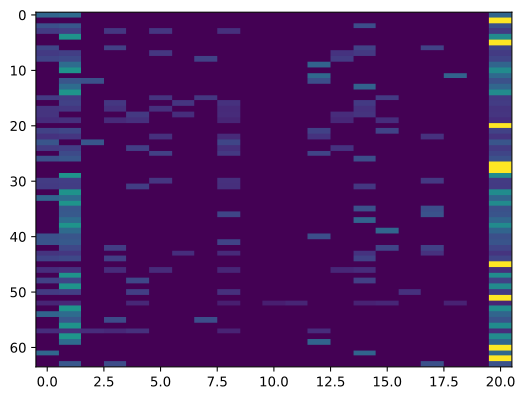
Except for the first two, our LFs usually abstain. Testing case where LF votes are all abstain:
p_all_abstain, _ = net(x_train["i=0:6000,d=7k"], -torch.ones_like(L_train["i=0:6000"]), p_gen, p_student)
(p_all_abstain == p_gen).all() # all abstain case: fallback to gen model probstensor(True)Teacher training
Teacher training minimizes two components of the loss: (1) minimum entropy regularization on a random batch B_U \subset D_U of the unlabeled pool pushes the teacher to produce confident (low-entropy) aggregated labels on the unlabeled pool by concentrating attention on voters that agree — effectively using voter consensus as unsupervised signal (with TF-IDF this sharpens noise; with BERT it sharpens genuine patterns), and (2) grounding (i.e. supervision) on a small labeled set D_L by minimizing cross-entropy against the true labels:
\mathcal{L}_{T} = -\frac{1}{|D_L|}\sum_{\textbf{\textsf{x}}_{i} \in D_L} \mathbf{e}_{y_i} \cdot \log \tilde{\textbf{\textsf{p}}}_{i} - \beta \frac{1}{|B_U|}\sum_{\textbf{\textsf{x}}_{i^{\prime}} \in B_U} \tilde{\textbf{\textsf{p}}}_{i^\prime} \cdot \log \tilde{\textbf{\textsf{p}}}_{i^\prime}
where \beta > 0 is weight on the entropy. Hence, the trainable parameters of the teacher network are for the query encoder \mathbf{W}_q and \mathbf{W}_k that consists of vectors to up-weight LFs that are reliable for the types of instances seen in D_L, and to down-weight noisy or irrelevant voters (including the student).
import copy
from tqdm.notebook import tqdm

def train_teacher(
    teacher, student_clf, gen_model,
    x_label, y_label, L_label,
    x_valid, y_valid, L_valid,
    x_pool=None, L_pool=None,
    epochs=150, lr=1e-3, alpha=1e-4,
    entropy_weight=0.2, pool_batch_size=512
):
    """Supervise the teacher on labeled examples with min-entropy on the unlabeled pool."""

    optim = torch.optim.Adam(teacher.parameters(), lr=lr, weight_decay=alpha)
    best_loss, best_state = float("inf"), None
    history = {"train": [], "valid": []}

    with torch.no_grad():
        # Precompute teacher inputs: (x, L, p_gen, p_student)
        p_gen_train = gen_model.predict_proba(L_label)
        p_gen_valid = gen_model.predict_proba(L_valid)
        p_student_train = torch.softmax(student_clf(x_label), dim=1)
        p_student_valid = torch.softmax(student_clf(x_valid), dim=1)

        # Precompute unlabeled inputs for entropy term
        if x_pool is not None:
            p_gen_u = gen_model.predict_proba(L_pool)
            p_student_u = torch.softmax(student_clf(x_pool), dim=1)

    patience = max(5, int(0.1 * epochs))
    bad_epochs = 0

    for _ in tqdm(range(epochs), desc="teacher", leave=False):
        agg_train, _ = teacher(x_label, L_label, p_gen_train, p_student_train)
        loss = F.nll_loss(torch.log(agg_train.clamp_min(1e-6)), y_label)

        # Min-entropy on unlabeled pool
        if x_pool is not None:
            idx_u = torch.randperm(x_pool.shape[0])[:pool_batch_size]
            agg_u, _ = teacher(x_pool[idx_u], L_pool[idx_u], p_gen_u[idx_u], p_student_u[idx_u])
            entropy = -(agg_u * torch.log(agg_u.clamp_min(1e-6))).sum(dim=1).mean()
            loss += entropy_weight * entropy

        history["train"].append(loss.item())

        optim.zero_grad()
        loss.backward()
        optim.step()

        with torch.no_grad():
            agg_val, _ = teacher(x_valid, L_valid, p_gen_valid, p_student_valid)
            val_loss = F.nll_loss(torch.log(agg_val.clamp_min(1e-6)), y_valid)

        history["valid"].append(val_loss.item())

        if val_loss.item() < best_loss:
            best_loss = val_loss.item()
            best_state = copy.deepcopy(teacher.state_dict())
            bad_epochs = 0
        else:
            bad_epochs += 1
            if bad_epochs >= patience:
                break

    if best_state is not None:
        teacher.load_state_dict(best_state)

    return history


def predict_teacher(teacher, student_clf, gen_model, x_all, L_all, batch_size=512):
    """Aggregate soft labels for the full training pool using the teacher."""
    teacher.eval()
    B = batch_size
    batches = []
    with torch.no_grad():
        for i in range(0, x_all.shape[0], B):
            xb, lb = x_all[i: i+B], L_all[i: i+B]
            agg, _ = teacher(xb, lb, gen_model.predict_proba(lb), torch.softmax(student_clf(xb), 1))
            batches.append(agg)

    teacher.train()
    return torch.cat(batches, dim=0)
ASTRA loop
Before the loop we do: (I) warm-start the student on NAT.v2 weights. Then, the ASTRA loop consists of: (L1) re-initialize the teacher6 since the small teacher network immediately saturates, halting further student progress, (L2) train the teacher with min-entropy on the unlabeled pool (sharpening attention using voter consensus) and fine-tune the teacher on labeled data (grounding) encapsulated within train_teacher, (L3) apply the teacher to the unlabeled pool to produce pseudo-labels, then perform confidence-weighted training for the student, and (L4) grounding the student via the usual hard-label training on the labeled dataset.
J = len(text_lfs)

# Creating LF outputs for the unlabeled pool since we need posterior probas for attn fallback.
L_valid["i=400:600"]    = build_L_text(text_lfs, valid_texts[400:600])
L_train["i=6000:16000"] = build_L_text(text_lfs, train_texts[6000:16000])
L_all = torch.cat([L_train["i=0:6000"],      L_train["i=6000:16000"]])          # (16000, J)
x_all = torch.cat([x_train["i=0:6000,d=7k"], x_train["i=6000:16000,d=7k"]])     # (16000, 7000)


# ── ASTRA loop ────────────────────────────────────────────────────────────────
N_ROUNDS       = 5
TEACHER_EPOCHS = 150
STUDENT_EPOCHS = 300
PSEUDO_CONF_THRESHOLD = 0.85

set_seed(RANDOM_SEED)

best_val_loss = float("inf")
1student_clf = make_student(NAT_V2_STATE)
astra_histories = []                                                              # per-round histories for plotting

for round_idx in range(N_ROUNDS):
    print(f"\n[Round {round_idx + 1}/{N_ROUNDS}]")

    # Re-initialize teacher each round so it adapts to the updated student
    teacher = RuleAttentionTeacher(n_features=7000, n_lfs=J, n_classes=K, hidden_dim=64, temperature=0.7)

    # Teacher: supervised on labeled set + min-entropy on unlabeled pool
    teacher_hist = train_teacher(
2        teacher, student_clf, gen_model_imdb,
        x_valid["i=400:600,d=7k"], y_valid["i=400:600"], L_valid["i=400:600"],
        x_valid["i=0:400,d=7k"], y_valid["i=0:400"], L_valid["i=0:400"],
        x_pool=x_all, L_pool=L_all,
        epochs=TEACHER_EPOCHS, lr=1e-3, alpha=1e-4,
        entropy_weight=0.003
    )

    # Student: train on teacher soft labels over full pool
    p_teacher_all = predict_teacher(teacher, student_clf, gen_model_imdb, x_all, L_all)
    conf_teacher = p_teacher_all.max(dim=1).values
    mask_teacher = conf_teacher >= PSEUDO_CONF_THRESHOLD

    x_pseudo = x_all[mask_teacher]
    p_pseudo = p_teacher_all[mask_teacher]
    w_pseudo = p_pseudo.max(dim=1).values
    print(f"(1) Pseudo-label training: ({int(mask_teacher.sum().item())}/{x_all.shape[0]} samples)")

    result_pseudo = train_cross_entropy(
        student_clf,
        x_pseudo, p_pseudo,
        x_valid["i=0:400,d=7k"], y_valid["i=0:400"],
        weights=w_pseudo,
        epochs=STUDENT_EPOCHS, bs=32, lr=3e-4, alpha=1e-3, momentum=0.9,
    )

    # Grounding: usual hard-label training on the 200 labeled examples
    print(f"\n(2) Grounding on labeled set: ({len(x_valid["i=400:600,d=7k"])} samples)")
    result_ground = train_cross_entropy(
        student_clf,
        x_valid["i=400:600,d=7k"], y_valid["i=400:600"],
        x_valid["i=0:400,d=7k"],   y_valid["i=0:400"],
        epochs=STUDENT_EPOCHS, bs=32, lr=3e-5, alpha=1e-3, momentum=0.9,
    )

    astra_histories.append({"teacher": teacher_hist, "pseudo": result_pseudo, "ground": result_ground})

    val_loss = result_ground["best_val_loss"]
    print("\n", f"  Round valid loss = {val_loss:.4f}")
3    if val_loss < best_val_loss:
        best_val_loss = val_loss
        best_state = copy.deepcopy(student_clf.state_dict())

# After ASTRA rounds, load best student model for final evaluation
astra_clf = make_student(best_state)- 1
- Student is warm-started from NAT v2 weights.
- 2
- Teacher trained with supervised loss + min-entropy regularization on the unlabeled pool.
- 3
-
Model selection across rounds uses best valid loss on the same
i=0:400validation set as all other methods.
seed: 0  deterministic: False

[Round 1/5]
(1) Pseudo-label training: (9209/16000 samples)Early stopping at epoch 40...
Training stopped.
Best train loss: 0.1663 | Best valid loss: 0.3989
(2) Grounding on labeled set: (200 samples)Best train loss: 0.1661 | Best valid loss: 0.3847
Round valid loss = 0.3847
[Round 2/5](1) Pseudo-label training: (9625/16000 samples)Early stopping at epoch 45...
Training stopped.
Best train loss: 0.1551 | Best valid loss: 0.3847
(2) Grounding on labeled set: (200 samples)Early stopping at epoch 288...
Training stopped.
Best train loss: 0.0992 | Best valid loss: 0.3787
Round valid loss = 0.3787
[Round 3/5](1) Pseudo-label training: (9790/16000 samples)Early stopping at epoch 69...
Training stopped.
Best train loss: 0.1469 | Best valid loss: 0.3785
(2) Grounding on labeled set: (200 samples)Early stopping at epoch 199...
Training stopped.
Best train loss: 0.0802 | Best valid loss: 0.3754
Round valid loss = 0.3754
[Round 4/5](1) Pseudo-label training: (10062/16000 samples)Early stopping at epoch 44...
Training stopped.
Best train loss: 0.1502 | Best valid loss: 0.3753
(2) Grounding on labeled set: (200 samples)Early stopping at epoch 52...
Training stopped.
Best train loss: 0.0856 | Best valid loss: 0.3726
Round valid loss = 0.3726
[Round 5/5](1) Pseudo-label training: (10148/16000 samples)Early stopping at epoch 36...
Training stopped.
Best train loss: 0.1553 | Best valid loss: 0.3735
(2) Grounding on labeled set: (200 samples)Early stopping at epoch 77...
Training stopped.
Best train loss: 0.0857 | Best valid loss: 0.3711
Round valid loss = 0.3711Loss curves over all ASTRA rounds. All three phases: teacher, student pseudo-label, and student grounding are shown. Each portion of the student grounding phase can be imagined to be sandwiched within a vertical line in the pseudo-label phase. Loss spikes in the teacher curve reflect re-initialization each round; though it nevertheless becomes progressively better.
Code
from notebooks.plot import Plot

# ── Aggregate histories ───────────────────────────────────────────────────────
teacher_train, teacher_valid = [], []
pseudo_train, pseudo_valid, pseudo_vsteps = [], [], []
ground_train, ground_valid, ground_vsteps = [], [], []
teacher_bounds, pseudo_bounds, ground_bounds = [], [], []
t_off, p_off, g_off = 0, 0, 0

for h in astra_histories:
    teacher_bounds.append(t_off)
    teacher_train.extend(h["teacher"]["train"])
    teacher_valid.extend(h["teacher"]["valid"])
    t_off += len(h["teacher"]["train"])

    pseudo_bounds.append(p_off)
    pseudo_train.extend(h["pseudo"]["train"])
    pseudo_valid.extend(h["pseudo"]["valid"])
    pseudo_vsteps.extend([s + p_off for s in h["pseudo"]["valid_steps"]])
    p_off += len(h["pseudo"]["train"])

    ground_bounds.append(g_off)
    ground_train.extend(h["ground"]["train"])
    ground_valid.extend(h["ground"]["valid"])
    ground_vsteps.extend([s + g_off for s in h["ground"]["valid_steps"]])
    g_off += len(h["ground"]["train"])

# ── Plot: 3 rows ─────────────────────────────────────────────────────────────
p = Plot(3, 1, figsize=(10, 9))

# Row 0 — Teacher (continuous, re-initialized each round)
p[0].line(teacher_train, color="C0", label="train")
p[0].line(teacher_valid, color="C1", label="valid")
for b in teacher_bounds[1:]:
    p[0].vline(b)
p[0].labels(x="epoch", y="loss", title="Teacher (re-initialized each round)")

# Row 1 — Student pseudo-label training (continuous)
p[1].line(pseudo_train, color="C0", label="train", smooth=50)
p[1].line(pseudo_valid, x=pseudo_vsteps, color="C1", label="valid")
for b in pseudo_bounds[1:]:
    p[1].vline(b)
p[1].labels(x="step", y="loss", title="Student — pseudo-label training")
p[1].ylim(0.0, 0.42)

# Row 2 — Student grounding (continuous)
p[2].line(ground_train, color="C0", label="train", smooth=50)
p[2].line(ground_valid, x=ground_vsteps, color="C1", label="valid")
for b in ground_bounds[1:]:
    p[2].vline(b)
p[2].labels(x="step", y="loss", title="Student — grounding (labeled)")
p[2].ylim(0.0, 0.42)

p.legend(loc="below")
p.show()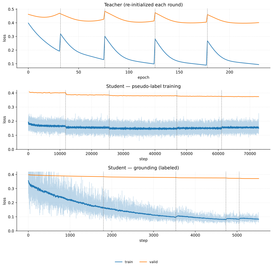
Comparing teacher attention weights before and after training. Observe that the teacher relies more on the student after the ASTRA training rounds. Recall that we drop using LFs for test inference, so this is good— it indicates that knowledge in the LFs have been properly distilled in the discriminative model, making the model sufficient by itself.
# Recall the student evolves with the teacher, so we use trained student preds
p_stu_final = torch.softmax(astra_clf(x_train["i=0:6000,d=7k"][:64]), dim=1).detach()
probs, attn_weights = teacher(x_train["i=0:6000,d=7k"][:64], L_train["i=0:6000"][:64], p_gen[:64], p_stu_final)
Code
fig, ax = plt.subplots(1, 2, figsize=(12, 4))
ax[0].set_title("Random teacher weights")
ax[1].set_title(f"Trained teacher weights (after {N_ROUNDS} rounds)")
ax[0].imshow(attn_weights0.cpu().detach().numpy(), aspect="auto");
ax[1].imshow(attn_weights.cpu().detach().numpy(), aspect="auto");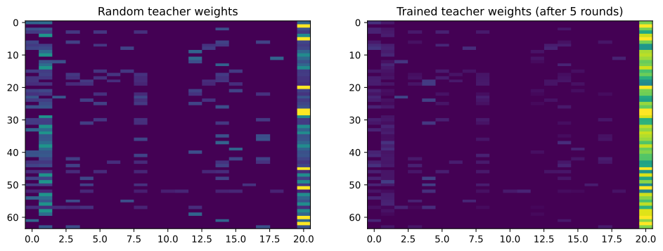
Note
Beyond TF-IDF: unlocking the attention mechanism. The trained attention weights above for the LFs are mostly zero because the query encoder — a single linear layer on sparse word counts — cannot learn fine-grained cues about when a given LF is reliable. With a pretrained language model encoder (e.g. BERT), the query \textbf{\textsf{q}}_i would capture context-dependent semantics (e.g. detecting sarcasm, quotation, negation), enabling the attention to meaningfully up-weight or down-weight voters per instance. Replacing the TF-IDF encoder with a pretrained language model backbone would be the natural next step to realize the full gains reported in the ASTRA paper.
Sigmoid attention with rule embeddings. The original ASTRA framework (Karamanolakis et al. 2021) replaces our masked softmax (where weights must sum to 1) with independent fidelity weights a_i^j = \sigma(f(\textbf{\textsf{h}}_i)^\top \textbf{\textsf{r}}_j) \in [0,1] per voter, where \textbf{\textsf{h}}_i is a feature representation from the BERT-based student7, f is a learned projection, and \textbf{\textsf{r}}_j is a learned embedding of LF j. Identically, a^S_i is calculated for the student with embedding \textbf{\textsf{r}}_S. Here \textbf{\textsf{h}}_i improves as the student trains across rounds, directly improving the teacher’s attention — this tight coupling is what enables co-evolution. The aggregated label becomes \tilde{\textbf{\textsf{p}}}_i = \frac{1}{Z_i}\big(\sum_{j \in R_i} a_i^j\, \textbf{\textsf{v}}_{ij} + a_i^S\, \hat{\textbf{\textsf{p}}}_{\Theta,i} + a_i^u\, \textbf{\textsf{u}}\big), where \textsf{u}_k \equiv 1/K is a uniform prior and a_i^u = (|R_i| - \sum_{j \in R_i} a_i^j) + (1 - a_i^S) is the residual weight (|R_i| = number of non-abstaining LFs for instance i), and Z_i is a normalization factor. Hence, when all fidelity weights are low the uniform dominates — the model expresses maximum uncertainty; when voters are trusted, it vanishes.
Evaluation. We report weighted F1 on the 400-sample validation set and the 2,000-sample oracle test set.
astra_pred = Predictor(astra_clf, K)

print("ASTRA — best student checkpoint")
r_val = evaluate(astra_pred, x_valid["i=0:400,d=7k"], y_valid["i=0:400"])
print(r_val["message"])

r_oracle = evaluate(astra_pred, x_oracle["i=0:2000,d=7k"], y_oracle["i=0:2000"], verbose=False)
print(r_oracle["message"])

# Baseline (NAT v2 + self-training)
b_val    = evaluate(predictor_ft, x_valid["i=0:400,d=7k"], y_valid["i=0:400"], verbose=False)
b_oracle = evaluate(predictor_ft, x_oracle["i=0:2000,d=7k"], y_oracle["i=0:2000"], verbose=False)
print()
print(f"ΔF1 pp. vs self-training + FT (valid):  {(r_val['f1']    - b_val['f1'])*100:+.2f}")
print(f"ΔF1 pp. vs self-training + FT (oracle): {(r_oracle['f1'] - b_oracle['f1'])*100:+.2f}")

# Store for results table
astra_valid  = r_val["f1"]
astra_oracle = r_oracle["f1"]
ASTRA — best student checkpoint
[[166 32]
[ 26 176]]
m=400, f1=0.85495, t=0.50000
m=2000, f1=0.85598, t=0.50000
ΔF1 pp. vs self-training + FT (valid): +0.51
ΔF1 pp. vs self-training + FT (oracle): +0.60\blacksquare
Appendix: Results Table
Comparing all variants on the IMDB validation set (400 labeled reviews, disjoint from training). Although standard practice, we can see that early stopping and validating on the same set yields generally optimistic estimates of improvement of performance from the baseline8. We know this by having a Oracle F1 column which reports performance on a held-out 2000-sample labeled test set, providing an unbiased estimate of generalization.
| Model | Features | Train Size | Valid Loss | Valid F1 | Oracle F1 | \Deltapp Valid | \Deltapp Oracle |
|---|---|---|---|---|---|---|---|
| GenModel (baseline) | LF outputs | 3,000 | — | 0.782 | — | — | — |
| NAT (baseline) | unigram TF-IDF (5k) | 3,000 | 0.408 | 0.822 | 0.827 | +0.0 | +0.0 |
| NAT v2 (base model only) | bigram TF-IDF (7k) | 6,000 | 0.402 | 0.837 | 0.835 | +1.5 | +0.8 |
| NAT baseline + self-training | unigram TF-IDF (5k) | 3,000 + pseudo | 0.399 | 0.825 | 0.830 | +0.3 | +0.4 |
| NAT v2 + self-training | bigram TF-IDF (7k) | 6,000 + pseudo | 0.393 | 0.837 | 0.847 | +1.5 | +2.0 |
| + fine-tuning (200 labels) | bigram TF-IDF (7k) | 6,000 + pseudo + 200 | 0.367 | 0.850 | 0.850 | +2.7 | +2.3 |
| ASTRA | bigram TF-IDF (7k) | 6,000 + pseudo + 200 | 0.371 | 0.855 | 0.856 | +3.3 | +2.9 |
| CE from scratch (200 labels) | bigram TF-IDF (7k) | 200 | 0.440 | 0.787 | 0.769 | -3.5 | -5.8 |
Both \Delta columns are relative to NAT (baseline). No model checkpoint, threshold, or architecture was selected based on the oracle set. The experiments and ablations show that improvement jointly comes from richer feature representations + increased data + model complexity, and the training methodology used (NAT -> self-training -> ASTRA).
Note
Q: Why is ~78% F1 from scratch still plausible? This highlights another aspect of the benefit having large amount of data, even when unlabeled (i.e. unsupervised learning). The classifier starts from random weights, but it does not start from raw text. Bigram TF-IDF is an unsupervised but already highly informative representation built from the full text corpus, so even 200 labeled reviews can be enough to learn a reasonable separation of obvious sentiment phrases such as waste of time, must watch, or highly recommend.
Appendix: (Not) Learning the Class Prior
Caution
Learning the prior from LF votes is unreliable. Unless the LFs are approximately symmetric across classes — similar coverage and accuracy for both classes — the learned prior will reflect LF vote skew rather than the true class balance. This is an unrealistic constraint in practice: LF developers naturally write rules that fire on the most discriminative signal, not rules that balance class counts. Treat this approach as an instructive exercise in extending GenModel, not a production recommendation.
Throughout the notebook we treated the class prior p_y as a fixed input. In practice, the true class balance is rarely known. One fix is to make p_y a learnable parameter and optimize it along with the confusion matrices via MLE. The only change required is in GenModel.fit where we introduce a logit vector \boldsymbol{\alpha} \in \mathbb{R}^K and compute p_y = \text{Softmax}(\boldsymbol{\alpha})_y at each step:
prior_logits = torch.nn.Parameter(torch.zeros(self.K))   # uniform init
optimizer = torch.optim.Adam([logits, prior_logits], lr=lr)

# Then inside the training loop:
self.py = torch.softmax(prior_logits, dim=0)
NOTE: The rest of the model (loss_fn, _build_C, predict) remains unchanged because they already reference self.py.
The intuition is that LF agreement patterns carry information about the class balance: if LFs vote positive more often, the marginal likelihood is higher under a prior that skews positive, so gradient descent will push \boldsymbol{\alpha} in that direction. However, this is also the failure mode. If the LFs themselves are asymmetric across classes (higher coverage or accuracy for one class), the learned prior absorbs LF bias rather than the true class balance.
We ran this experiment9 and obtained the following results:
| Experiment | True prior | Learned prior | Fixed-prior F1 | Learned-prior F1 |
|---|---|---|---|---|
| Synthetic | 0.40 / 0.60 | 0.37 / 0.63 | 0.777 | 0.777 |
| IMDB | 0.50 / 0.50 | 0.31 / 0.69 | 0.770 | 0.712 |
On synthetic data, the learned prior is close to ground truth, and F1 is comparable. On IMDB, lf_sentiment_words correctly labels 875 positives but only 485 negatives, so the MLE prior absorbs the LF skew and F1 drops by several points. The root cause is an identifiability problem: the marginal likelihood p(\Lambda) = \sum_y p_y \prod_j C^j_{y,\lambda_j} cannot distinguish LF bias from true class imbalance: C^j_{y,\lambda_j} = p_\Phi(\lambda_j \mid y) is conditioned on y — so it doesn’t care about p_y, while p_y is incentivized to amplify LF bias to maximize p(\Lambda).
Indeed, dropping lf_sentiment_words does not recover 0.50; it collapses the prior to the opposite extreme (0.999/0.001) because the remaining LFs are collectively negative-biased. A single dominant LF can flip the learned prior entirely.
Tip
A small labeled sample is a more robust alternative to learning the prior from LF votes. As shown above, the learned prior is unreliable unless LFs are symmetric across classes — a constraint that conflicts with how LFs are naturally developed. Even 50–100 labels can beat a badly learned prior, as the CI analysis below shows. In general, getting more samples help to reduce CI width at the rate O(1/{\sqrt{n}}). More details below.
How many labels do you need? Suppose you hand-label n examples and find that a fraction \hat{p} of them are positive. Then, the 95% confidence interval10 (CI) for the true positive fraction p is approximately \hat{p} \pm 1.96\sqrt{\hat{p}(1-\hat{p})/n}. The interval is widest when \hat{p} = 0.5 (balanced classes), which gives an upper bound on how imprecise your estimate can be:

| Labeled samples n | 95% CI half-width | Example: \hat{p} = 0.50 |
|---|---|---|
| 30 | \pm 0.18 | [0.32, 0.68] |
| 50 | \pm 0.14 | [0.36, 0.64] |
| 100 | \pm 0.10 | [0.40, 0.60] |
| 200 | \pm 0.07 | [0.43, 0.57] |
| 500 | \pm 0.04 | [0.46, 0.54] |
So 50–100 labels give you roughly \pm 0.10–0.14 precision on the prior. Whether that’s good enough depends on how wrong the alternative is. In our IMDB case the learned prior was off by 0.19 (0.31 vs. 0.50), so even 50 labeled examples would likely beat it. But if the LFs were only slightly biased, a noisy 50-sample estimate could be worse.
References
Karamanolakis, Giannis, Subhabrata Mukherjee, Guoqing Zheng, and Ahmed Hassan Awadallah. 2021. “Self-Training with Weak Supervision.” CoRR abs/2104.05514. https://arxiv.org/abs/2104.05514.
Ratner, Alexander, Christopher De Sa, Sen Wu, Daniel Selsam, and Christopher Ré. 2017. Data Programming: Creating Large Training Sets, Quickly. https://arxiv.org/abs/1605.07723.
Footnotes
See Text-to-LoRA. Also the ProgramAsWeights project which compiles an LLM into task-specific runnable local functions.↩︎
While we need p_{\hat{\Phi}}(y \mid \lambda_\textbf{\textsf{x}}) for training, what we have access to is the reverse: p_{\hat{\Phi}}(\lambda_\textbf{\textsf{x}} \mid y) which we estimate by performing MLE on the LF outputs based on all targets (since we don’t know which is the real one).↩︎
Recall that the five simulated LFs have F1 ranging from 0.66 to 0.90, with coverages of 20–50%. In particular, LF5 has the highest F1 at 0.92, but fires on only 25% of examples.↩︎
Retraining
GenModelon the larger set actually hurts performance, our guess is that the additional data dilutes the LF statistics the model was optimized on (we have too few parameters for 6000 data points).↩︎For instance, lf_rating_mention is highly reliable when a reviewer writes “10/10” sincerely, but misleading when the same pattern appears in a dismissive context (e.g. “the poster said 10/10 but this was garbage”) — the generative model treats the LF identically in both cases.↩︎
Drifts from our above discussion of pure co-evolution, but is necessary to get good performance.↩︎
For a BERT-based student \textbf{\textsf{h}}_i is the penultimate hidden layer output; for simpler models it is the raw input embedding — exactly as in our TF-IDF setup. In our simplified implementation we use raw TF-IDF features rather than student hidden states, since the shallow MLP student provides limited representation quality.↩︎
That is, we generally have \Deltapp Valid \geq \Deltapp Oracle. The former is the observed improvements in the experiments, while the latter is the latent or “true” improvement that we don’t have access to.↩︎
Same params
epochs=5000,lr=0.01and datasetsL_train,L_valid.↩︎A 95% confidence interval means that if you repeated this sampling-and-estimation procedure many times, about 95% of the resulting intervals would contain the true parameter.
Operationally, if you collect 100 labeled samples and compute the interval, you can act as if the true prior lies within it — accepting a 1-in-20 chance of being wrong. Note that the prior affects both training and inference, so errors compound: if your LFs are already somewhat positive-biased, an overestimated prior amplifies that bias further through training, then again at inference.↩︎