import numpy as np
import matplotlib.pyplot as plt

rng = np.random.default_rng(42)
theta_true = 5.0
n = 50
data = rng.uniform(0, theta_true, size=n)
x_max = data.max()Maximum Likelihood Estimation
statistics
probability
machine-learning
Introduction
Maximum likelihood estimation (MLE) is a way to estimate unknown parameters from observed data. Given a probabilistic model and observations x_1, \ldots, x_n, MLE chooses the parameter value under which those observations are most plausible.
The recipe is simple: write the joint density of the data as a function of the parameter, then maximize it. This note develops the recipe for a deliberately instructive model, X_i \stackrel{\text{iid}}{\sim} \text{Uniform}(0, \theta). The example shows why the support of a distribution matters, why an MLE can occur at a boundary rather than at a stationary point, and why maximum likelihood does not guarantee an unbiased estimator.
The model
Let
X_1, \ldots, X_n \stackrel{\text{iid}}{\sim} \text{Uniform}(0, \theta), \qquad \theta > 0,
where \theta is unknown. The density is
f(x; \theta) = \begin{cases} 1/\theta, & 0 \leq x \leq \theta, \\ 0, & \text{otherwise}. \end{cases}
The population mean and variance are \mathbb{E}[X] = \theta/2 and \operatorname{Var}(X) = \theta^2/12. More importantly for MLE, the support depends on \theta. If the observed sample has maximum
x_{(n)} = \max(x_1, \ldots, x_n),
then every admissible value of \theta must satisfy \theta \geq x_{(n)}. A candidate below the sample maximum assigns zero density to an observed value.
A synthetic sample
Draw 50 observations from \text{Uniform}(0, 5) and keep the true upper bound hidden from the estimation step:
Code
fig, ax = plt.subplots(figsize=(8, 3))
ax.hist(data, bins=15, density=True, alpha=0.7, color="C0")
ax.axvline(theta_true, color="C1", linestyle="--", label=r"true $\theta = 5$")
ax.axvline(x_max, color="C2", linestyle=":", label=r"observed max $x_{(n)}$")
ax.set_xlabel("x")
ax.set_ylabel("density")
ax.legend()
plt.show()

print(f"n = {n}, true theta = {theta_true:.1f}")
print(f"sample mean = {data.mean():.4f}")
print(f"sample max  = {x_max:.4f}")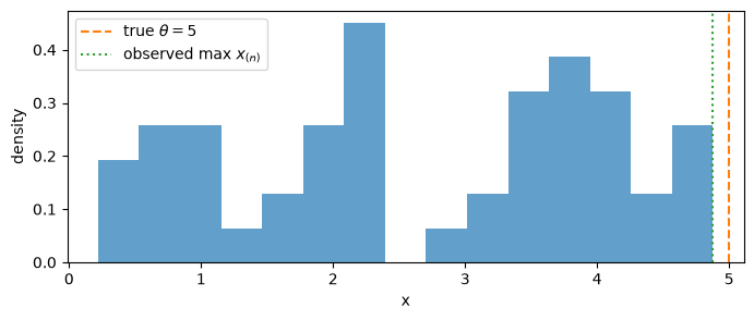
n = 50, true theta = 5.0
sample mean = 2.6762
sample max  = 4.8781
The observed maximum falls short of the true upper bound, which is typical for a finite sample. The missing interval (x_{(n)}, \theta] contains no observations, but it still belongs to the data-generating distribution. The likelihood will decide how much of that unobserved interval to retain.
The likelihood
For a fixed observed sample \boldsymbol{x} = (x_1, \ldots, x_n), the likelihood treats the data as fixed and the parameter as variable:
L(\theta; \boldsymbol{x}) = \prod_{i=1}^n f(x_i; \theta) = \theta^{-n}\, \mathbb{1}\!\left[\theta \geq x_{(n)}\right].
The indicator records the support constraint. For every admissible \theta \geq x_{(n)},
\ell(\theta; \boldsymbol{x}) = \log L(\theta; \boldsymbol{x}) = -n \log \theta.
Maximizing the likelihood or the log-likelihood gives the same answer because the logarithm is strictly increasing. The log form is usually easier to work with because products become sums.
Evaluate the log-likelihood over a grid of candidate upper bounds. The vertical lines show the true parameter and the point where the likelihood first becomes nonzero:
theta_grid = np.linspace(0.5, 6.5, 600)
log_likelihood = np.where(
    theta_grid >= x_max,
    -n * np.log(theta_grid),
    -np.inf,
)
Code
fig, ax = plt.subplots(figsize=(8, 3))
ax.plot(theta_grid, log_likelihood, color="C0")
ax.axvline(theta_true, color="C1", linestyle="--", label=r"true $\theta$")
ax.axvline(x_max, color="C2", linestyle=":", label=r"$x_{(n)}$")
ax.set_xlabel(r"candidate $\theta$")
ax.set_ylabel(r"$\ell(\theta; \boldsymbol{x})$")
ax.legend()
plt.show()

print(f"likelihood is zero for theta < {x_max:.4f}")
print(f"analytic maximizer = {x_max:.4f}")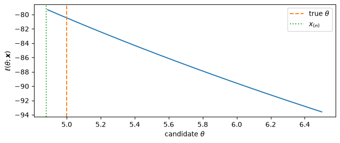
likelihood is zero for theta < 4.8781
analytic maximizer = 4.8781
Deriving the MLE
The likelihood is zero whenever \theta < x_{(n)}. On the admissible region,
\ell(\theta; \boldsymbol{x}) = -n\log\theta, \qquad \frac{\mathrm{d}}{\mathrm{d}\theta}\ell(\theta; \boldsymbol{x}) = -\frac{n}{\theta} < 0.
Thus the log-likelihood is strictly decreasing over every admissible value. Its maximum is attained at the smallest admissible value:
\boxed{\widehat{\theta}_{\mathrm{MLE}} = x_{(n)} = \max_i x_i}.
There is no interior critical point to solve for. This is a useful warning: differentiating the log-likelihood is effective for many regular models, but it does not replace checking the parameter space and its boundaries.
Finite-sample behavior
The MLE is feasible, but it is not unbiased. The distribution of the sample maximum follows directly from independence. For 0 \leq t \leq \theta,
\Pr(X_{(n)} \leq t) = \Pr(X_1 \leq t, \ldots, X_n \leq t) = \left(\frac{t}{\theta}\right)^n.
Equivalently, X_{(n)}/\theta \sim \operatorname{Beta}(n, 1), so
\mathbb{E}[X_{(n)}] = \frac{n}{n+1}\theta, \qquad \operatorname{Bias}(\widehat{\theta}_{\mathrm{MLE}}) = -\frac{\theta}{n+1}.
The bias disappears as n grows, which makes the MLE consistent. If unbiasedness is important, the sampling distribution suggests the corrected estimator
\widehat{\theta}_{\mathrm{corr}} = \frac{n+1}{n} X_{(n)}, \qquad \mathbb{E}[\widehat{\theta}_{\mathrm{corr}}] = \theta.
Bias correction does not make the corrected estimator an MLE. It is a different estimator constructed using the finite-sample behavior of the MLE.
The following simulation compares the raw MLE with the bias-corrected estimator across repeated samples. The corrected estimator should average close to the true value, while the raw MLE should approach it from below:
sample_sizes = np.array([2, 5, 10, 25, 50, 100])
n_reps = 10_000
sim_rng = np.random.default_rng(7)

mle_means = []
corrected_means = []

1for sample_size in sample_sizes:
2    samples = sim_rng.uniform(
        0, theta_true, size=(n_reps, sample_size)
    )
3    maxima = samples.max(axis=1)
4    mle_means.append(maxima.mean())
5    corrected_means.append(
        ((sample_size + 1) / sample_size * maxima).mean()
)- 1
- Repeat the experiment for each sample size so the finite-sample trend is visible.
- 2
- Draw independent samples from the true \text{Uniform}(0, \theta) distribution.
- 3
- Reduce each repeated sample to its maximum, the MLE for this model.
- 4
- Average the raw MLEs to estimate their expected value.
- 5
- Apply the exact finite-sample correction before averaging the corrected estimates.
Code
fig, ax = plt.subplots(figsize=(8, 3.5))
ax.plot(sample_sizes, mle_means, "o-", label="MLE")
ax.plot(sample_sizes, corrected_means, "o-", label="bias-corrected")
ax.axhline(theta_true, color="C2", linestyle="--", label=r"true $\theta$")
ax.set_xscale("log")
ax.set_xlabel("sample size (log scale)")
ax.set_ylabel("average estimate")
ax.legend()
plt.show()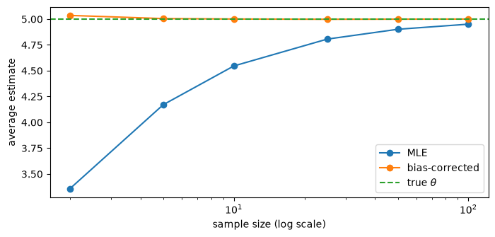
Code
from IPython.display import Markdown, display

table = [
    "| n | average MLE | theoretical MLE | average corrected |",
    "|---:|---:|---:|---:|",
]

for sample_size, mle_mean, corrected_mean in zip(
    sample_sizes, mle_means, corrected_means
):
    theoretical = sample_size / (sample_size + 1) * theta_true
    table.append(
        f"| {sample_size} | {mle_mean:.4f} | "
        f"{theoretical:.4f} | {corrected_mean:.4f} |"
    )

display(Markdown("\n".join(table)))| n | average MLE | theoretical MLE | average corrected |
|---|---|---|---|
| 2 | 3.3571 | 3.3333 | 5.0357 |
| 5 | 4.1709 | 4.1667 | 5.0050 |
| 10 | 4.5463 | 4.5455 | 5.0009 |
| 25 | 4.8063 | 4.8077 | 4.9986 |
| 50 | 4.9015 | 4.9020 | 4.9995 |
| 100 | 4.9510 | 4.9505 | 5.0005 |
The simulation matches the exact calculation:
| Estimator | Expression | Finite-sample behavior |
|---|---|---|
| MLE | X_{(n)} | Feasible, downward biased, consistent |
| Bias-corrected | \frac{n+1}{n}X_{(n)} | Unbiased, consistent, can overshoot \theta |
Note
This is a nonregular MLE problem because the support changes with \theta. In regular models, such as a normal model with fixed support, the MLE is often found by setting the score (the derivative of the log-likelihood) to zero. Here the score is always negative on the admissible region, and the answer comes from the boundary.
Takeaways
Maximum likelihood turns a probabilistic model into an estimation procedure:
- Write the joint density as a function of the unknown parameter.
- Identify the parameter values allowed by the support of the observations.
- Maximize the likelihood, usually through its log.
- Check the result for bias, consistency, and other finite-sample properties.
For the uniform upper-bound model, the support constraint forces \theta \geq \max_i x_i, while the likelihood decreases as \theta increases. The maximum therefore occurs at the sample maximum:
\boxed{\widehat{\theta}_{\mathrm{MLE}} = \max_i x_i}.
The same logic applies to more complicated models. The main difference is that the final maximization may require algebra, numerical optimization, or a specialized algorithm.