from watchtower.core import set_format
set_format("svg")Foundations
This chapter fixes the object model and the notation the rest of the course relies on. A vector is a point in \mathbb{R}^n, a matrix is the representation of a linear map \mathbb{R}^n \to \mathbb{R}^m, and a norm is the ruler used to measure both. The three are introduced together because they are used together: every statement about a matrix is, in the end, a statement about what it does to the lengths and angles of vectors.
One convention carries through the whole course. Operators — linear maps, basis-free — are written in regular font (T, S); vectors and matrices, their concrete representations, are written in bold (\mathbf{x}, \mathbf{A}). The distinction marks exactly where a basis has been chosen. A vector is a column vector \mathbf{x} = (x_1, \dots, x_n)^{\mathsf T} \in \mathbb{R}^n; the transpose \mathbf{x}^{\mathsf T} is a row vector, and the standard inner product is \langle \mathbf{x}, \mathbf{y}\rangle = \mathbf{x}^{\mathsf T}\mathbf{y}. The field is \mathbb{R} throughout: everything is real unless the complex case is explicitly flagged, in which case each transpose becomes a conjugate transpose.
Vectors and their combinations
A vector space over \mathbb{R} is a set V equipped with addition V \times V \to V and scalar multiplication \mathbb{R} \times V \to V satisfying the standard axioms: associativity, commutativity, distributivity, and the existence of a zero vector and additive inverses. The working examples are \mathbb{R}^n and its subspaces.
Given vectors \mathbf{v}_1, \dots, \mathbf{v}_k \in V and scalars c_1, \dots, c_k, the expression \sum_{i=1}^k c_i \mathbf{v}_i is a linear combination of the \mathbf{v}_i. The set of all such combinations is the span of the list, written \operatorname{span}\{\mathbf{v}_1, \dots, \mathbf{v}_k\}; it is the smallest subspace containing every \mathbf{v}_i.
A list \mathbf{v}_1, \dots, \mathbf{v}_k is linearly independent if the only way to write \mathbf{0} as a linear combination is with every coefficient zero:
\sum_{i=1}^k c_i \mathbf{v}_i = \mathbf{0} \;\Longrightarrow\; c_1 = \cdots = c_k = 0 .
Equivalently, no vector in the list is a linear combination of the others: each \mathbf{v}_i contributes a genuinely new direction. If some nonzero combination sums to \mathbf{0} the list is linearly dependent.
A basis of V is a linearly independent list that spans V. Every vector then has a unique expansion in the basis; uniqueness fails exactly when the list is dependent. The dimension \dim V is the number of vectors in any basis, and every basis of a given space has the same number of vectors. The basis that makes everything concrete is the standard basis \mathbf{e}_1, \dots, \mathbf{e}_n of \mathbb{R}^n, where \mathbf{e}_i has a single 1 in position i; a vector \mathbf{x} is then the column of its coordinates, \mathbf{x} = \sum_i x_i \mathbf{e}_i.
Matrices are representations of linear maps
An operator is a linear map T : \mathbb{R}^n \to \mathbb{R}^m:
T(\alpha \mathbf{x} + \beta \mathbf{y}) = \alpha\, T(\mathbf{x}) + \beta\, T(\mathbf{y}) \qquad\text{for all } \mathbf{x}, \mathbf{y} \in \mathbb{R}^n,\ \alpha, \beta \in \mathbb{R}.
The operator is the geometric object; a matrix is its representation. Choosing the standard basis pins T to a unique m \times n matrix \mathbf{A} whose column j is T(\mathbf{e}_j), the image of the j-th basis vector. Then T(\mathbf{x}) = \mathbf{A}\mathbf{x} for every \mathbf{x}. An operator and its matrix are thus two views of one object: the operator is coordinate-free, the matrix is the operator in the standard coordinates, which is exactly the content of the notation \mathbf{A} \in \mathbb{R}^{m \times n} — \mathbf{A} takes an n-vector and returns an m-vector.
Composition is matrix multiplication. If T : \mathbb{R}^p \to \mathbb{R}^n is represented by the n \times p matrix \mathbf{B} and S : \mathbb{R}^n \to \mathbb{R}^m by the m \times n matrix \mathbf{A}, then the composite S \circ T is represented by the m \times p matrix \mathbf{A}\mathbf{B}, and (\mathbf{A}\mathbf{B})\mathbf{x} = \mathbf{A}(\mathbf{B}\mathbf{x}): multiplication by \mathbf{B} comes first, then by \mathbf{A}. The inner dimension n must match, the algebraic echo of the requirement that the range of T lie inside the domain of S.
Four ways to read \mathbf{A}\mathbf{B}
The product \mathbf{C} = \mathbf{A}\mathbf{B}, with \mathbf{A} \in \mathbb{R}^{m \times n} and \mathbf{B} \in \mathbb{R}^{n \times p}, can be assembled in four ways, each of which matters somewhere later in the course:
- Column combination. Column j of \mathbf{C} is \mathbf{A} applied to column j of \mathbf{B}: \mathbf{c}_j = \mathbf{A}\mathbf{b}_j = \sum_{i=1}^n b_{ij}\mathbf{a}_i, a linear combination of the columns of \mathbf{A}. The columns of \mathbf{C} are the images of the columns of \mathbf{B} under \mathbf{A}.
- Row combination. Row i of \mathbf{C} is a linear combination of the rows of \mathbf{B}: \mathbf{c}_i^{\mathsf T} = \sum_{k=1}^n a_{ik} \mathbf{b}_k^{\mathsf T}.
- Dot products. c_{ij} = \sum_{k=1}^n a_{ik} b_{kj}, the entrywise form. Right for hand computation, and the least geometric.
- Sum of rank-one outer products. With \mathbf{a}_k the k-th column of \mathbf{A} and \mathbf{b}_k^{\mathsf T} the k-th row of \mathbf{B},
\mathbf{C} = \sum_{k=1}^n \mathbf{a}_k \mathbf{b}_k^{\mathsf T}.
Each term is a rank-one matrix (all columns scalar multiples of \mathbf{a}_k). This view decomposes \mathbf{C} into n rank-one pieces and is the one that generalizes to the singular value decomposition in chapter 3.
Views 1 and 4 are the load-bearing ones. View 1 reads multiplication by \mathbf{A} as an action on columns; view 4 reads a product as a sum of simple pieces.
import numpy as np

rng = np.random.default_rng(1)
m, n, p = 3, 4, 2
A = rng.normal(size=(m, n))
B = rng.normal(size=(n, p))

AB = A @ B

# view 4: sum of rank-one outer products a_k b_k^T
outer = sum(np.outer(A[:, k], B[k, :]) for k in range(n))

# view 1: column j of AB is A applied to column j of B
col0 = A @ B[:, 0]

print("outer-sum equals AB   :", np.allclose(AB, outer))
print("column view equals AB :", np.allclose(AB[:, 0], col0))
print("rank-one term count   :", n)
outer-sum equals AB : True
column view equals AB : True
rank-one term count : 4The two views are not different algorithms so much as different readings of the same sum; the code confirms both identities to floating-point precision. Which view to use is a matter of which interpretation the argument at hand calls for. View 4 returns in earnest when every matrix in the course is expressed as a sum of rank-one pieces weighted by its singular values.
Inner product, orthogonality, Cauchy–Schwarz
The standard inner product (dot product) on \mathbb{R}^n is
\langle \mathbf{x}, \mathbf{y}\rangle = \mathbf{x}^{\mathsf T}\mathbf{y} = \sum_{i=1}^n x_i y_i .
It is bilinear, symmetric, and positive definite: \langle \mathbf{x}, \mathbf{x}\rangle \ge 0 with equality only at \mathbf{x} = \mathbf{0}. The Euclidean norm is \lVert \mathbf{x}\rVert = \sqrt{\langle \mathbf{x}, \mathbf{x}\rangle}.
Two vectors are orthogonal if \langle \mathbf{x}, \mathbf{y}\rangle = 0, written \mathbf{x} \perp \mathbf{y}. Orthogonality is the algebraic form of “no shared component”; it is the notion on which projection, and later the entire spectral theory, is built.
Cauchy–Schwarz. For all \mathbf{x}, \mathbf{y} \in \mathbb{R}^n,
|\langle \mathbf{x}, \mathbf{y}\rangle| \le \lVert \mathbf{x}\rVert\, \lVert \mathbf{y}\rVert,
with equality if and only if \mathbf{x} and \mathbf{y} are collinear.
Proof. For any real t the squared norm is nonnegative:
0 \le \lVert \mathbf{x} - t\mathbf{y}\rVert^2 = \langle \mathbf{x} - t\mathbf{y}, \mathbf{x} - t\mathbf{y}\rangle = \lVert \mathbf{x}\rVert^2 - 2t\langle \mathbf{x},\mathbf{y}\rangle + t^2 \lVert \mathbf{y}\rVert^2 .
For \mathbf{y} = \mathbf{0} the claim is trivial, so take \mathbf{y} \neq \mathbf{0}. The right-hand side is a quadratic in t with positive leading coefficient \lVert \mathbf{y}\rVert^2; its minimum occurs at t = \langle \mathbf{x},\mathbf{y}\rangle / \lVert \mathbf{y}\rVert^2, where its value is
\lVert \mathbf{x}\rVert^2 - \frac{\langle \mathbf{x},\mathbf{y}\rangle^2}{\lVert \mathbf{y}\rVert^2} \;\ge\; 0,
which rearranges to the stated bound. Equality forces \lVert \mathbf{x} - t\mathbf{y}\rVert = 0, hence \mathbf{x} = t\mathbf{y}: the vectors are collinear. \square
Two consequences matter immediately. First, the triangle inequality \lVert \mathbf{x} + \mathbf{y}\rVert \le \lVert \mathbf{x}\rVert + \lVert \mathbf{y}\rVert follows by expanding \lVert \mathbf{x}+\mathbf{y}\rVert^2 and applying Cauchy–Schwarz. Second, for nonzero \mathbf{x}, \mathbf{y} the quantity
\cos\theta = \frac{\langle \mathbf{x}, \mathbf{y}\rangle} {\lVert \mathbf{x}\rVert\,\lVert \mathbf{y}\rVert}
lies in [-1, 1], so it defines a genuine angle \theta between the two vectors.1
rng = np.random.default_rng(4)
x = rng.normal(size=50)
y = rng.normal(size=50)

lhs = abs(x @ y)
rhs = np.linalg.norm(x) * np.linalg.norm(y)

print("|<x,y>|            =", lhs)
print("||x|| ||y||         =", rhs)
print("ratio  (<= 1)       =", lhs / rhs)
print("angle  (radians)    =", np.arccos(np.clip(x @ y / rhs, -1, 1)))
|<x,y>| = 7.567879438125613
||x|| ||y|| = 51.40865076301386
ratio (<= 1) = 0.14721023263209917
angle (radians) = 1.4230491460386565The ratio |\langle \mathbf{x},\mathbf{y}\rangle| / (\lVert \mathbf{x}\rVert\lVert \mathbf{y}\rVert) is the absolute cosine of the angle; Cauchy–Schwarz is the statement that this ratio never exceeds 1. The bound is typically not tight: two random vectors in high dimension are nearly orthogonal, so the ratio is close to 0 rather than 1. Tightness is reserved for collinear vectors, which in \mathbb{R}^{50} are a measure-zero set. This gap between the generic case and the extremal case is a recurring theme: worst-case bounds in high dimension are almost never attained.
Norms
A norm on a vector space V is a map \lVert\cdot\rVert : V \to \mathbb{R}_{\ge 0} satisfying three properties:
- Positive definite: \lVert \mathbf{x}\rVert = 0 if and only if \mathbf{x} = \mathbf{0}.
- Homogeneous: \lVert \alpha \mathbf{x}\rVert = |\alpha|\, \lVert \mathbf{x}\rVert.
- Triangle inequality: \lVert \mathbf{x} + \mathbf{y}\rVert \le \lVert \mathbf{x}\rVert + \lVert \mathbf{y}\rVert.
Three norms on \mathbb{R}^n recur:
| Norm | Definition | Measures |
|---|---|---|
| \ell_1 | \lVert \mathbf{x}\rVert_1 = \sum_i |x_i| | total absolute mass; “taxicab” distance |
| \ell_2 | \lVert \mathbf{x}\rVert_2 = \big(\sum_i x_i^2\big)^{1/2} | Euclidean length |
| \ell_\infty | \lVert \mathbf{x}\rVert_\infty = \max_i |x_i| | largest coordinate magnitude |
Each is a legitimate norm, but they measure different things, and the differences are visible in their unit balls \{\mathbf{x} : \lVert \mathbf{x}\rVert \le 1\}. The figure draws the boundaries of these balls, the unit spheres \{\mathbf{x} : \lVert \mathbf{x}\rVert = 1\}.
import matplotlib.pyplot as plt
import numpy as np

t = np.linspace(0, 2 * np.pi, 2000)
circle = np.c_[np.cos(t), np.sin(t)]          # x with ||x||_2 = 1

def to_l1(x):                                 # rescale so ||x||_1 = 1
    return x / np.abs(x).sum(axis=1, keepdims=True)

def to_linf(x):                               # rescale so ||x||_inf = 1
    return x / np.abs(x).max(axis=1, keepdims=True)

balls = [
    (to_l1(circle),   r"$\ell_1$"),
    (circle,          r"$\ell_2$"),
    (to_linf(circle), r"$\ell_\infty$"),
]

fig, axes = plt.subplots(1, 3, figsize=(11, 3.8))
for ax, (pts, label) in zip(axes, balls):
    ax.plot(pts[:, 0], pts[:, 1], lw=2.2, color="#1f77b4")
    ax.set_aspect("equal")
    ax.set_title(label, fontsize=13)
    ax.grid(alpha=0.25)
    for spine in ("top", "right"):
        ax.spines[spine].set_visible(False)
    ax.axhline(0, color="k", lw=0.6)
    ax.axvline(0, color="k", lw=0.6)
plt.tight_layout()
plt.show()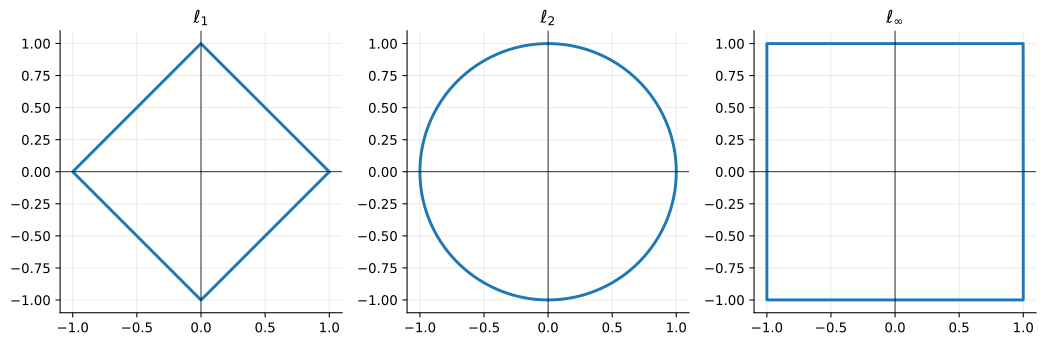
The \ell_1 ball is a diamond, the \ell_\infty ball a square, and only the \ell_2 ball is round. The roundness is not cosmetic: it is why the \ell_2 norm is the one tied to inner products and hence to orthogonality, angles, and the whole spectral theory. The diamond and the square have flat faces, which is what makes \ell_1 and \ell_\infty natural for sparse and robust problems in optimization; the course returns to this contrast in the least squares chapter.
All norms are equivalent in finite dimension
The three norms disagree on individual vectors, but not by much: in \mathbb{R}^n any two norms bound each other up to constants.
Norm equivalence. For any two norms \lVert\cdot\rVert_a and \lVert\cdot\rVert_b on \mathbb{R}^n there exist constants 0 < c \le C such that
c\,\lVert \mathbf{x}\rVert_b \le \lVert \mathbf{x}\rVert_a \le C\,\lVert \mathbf{x}\rVert_b \qquad\text{for all } \mathbf{x} \in \mathbb{R}^n .
For the three standard norms the constants are explicit. Cauchy–Schwarz with the all-ones vector gives \lVert \mathbf{x}\rVert_1 \le \sqrt{n}\,\lVert \mathbf{x}\rVert_2, and \lVert \mathbf{x}\rVert_2 \le \lVert \mathbf{x}\rVert_1 is immediate, so
\lVert \mathbf{x}\rVert_2 \le \lVert \mathbf{x}\rVert_1 \le \sqrt{n}\,\lVert \mathbf{x}\rVert_2 .
Similarly \lVert \mathbf{x}\rVert_\infty \le \lVert \mathbf{x}\rVert_2 \le \sqrt{n}\,\lVert \mathbf{x}\rVert_\infty and \lVert \mathbf{x}\rVert_\infty \le \lVert \mathbf{x}\rVert_1 \le n\,\lVert \mathbf{x}\rVert_\infty.
The analytic content is that convergence is norm-independent: a sequence converges in one norm if and only if it converges in every norm. But the constants matter numerically, and they grow with dimension. A vector that is “small” in \ell_\infty can be \sqrt{n} times larger in \ell_2 and n times larger in \ell_1, so “small” must always name its norm.
rng = np.random.default_rng(3)
X = rng.normal(size=(20000, 10))

n1 = np.abs(X).sum(axis=1)
n2 = np.linalg.norm(X, axis=1)
ninf = np.abs(X).max(axis=1)

print("max ||x||_1 / ||x||_2   =", (n1 / n2).max(),   "  theory:", np.sqrt(10))
print("max ||x||_2 / ||x||_inf =", (n2 / ninf).max(), "  theory:", np.sqrt(10))
print("max ||x||_1 / ||x||_inf =", (n1 / ninf).max(), "  theory:", 10)
max ||x||_1 / ||x||_2 = 3.1093448476542593 theory: 3.1622776601683795
max ||x||_2 / ||x||_inf = 2.6889665849668547 theory: 3.1622776601683795
max ||x||_1 / ||x||_inf = 8.287987254201049 theory: 10Over twenty thousand random vectors in \mathbb{R}^{10}, the largest observed ratios sit just below the theoretical ceilings \sqrt{10} and 10. The ceilings are attained only by vectors aligned with the extremal directions: the all-ones vector saturates all three ceilings (\sqrt{n} for the \ell_1/\ell_2 and \ell_2/\ell_\infty ratios, n for \ell_1/\ell_\infty), while the floors of 1 are attained by standard basis vectors. Random vectors come close without ever hitting them. These constants are not theoretical artifacts: they are the actual worst-case amplification between norms, and they set the scale in condition numbers later.
Matrix norms
Matrices form a vector space, so the vector-norm machinery applies to them directly, but two matrix norms dominate in practice.
The Frobenius norm is the \ell_2 norm of the entries flattened:
\lVert \mathbf{A}\rVert_F = \Big(\sum_{i,j} a_{ij}^2\Big)^{1/2} = \sqrt{\operatorname{tr}(\mathbf{A}^{\mathsf T}\mathbf{A})} .
It is the simplest norm, and it is invariant under orthogonal transformations: \lVert \mathbf{Q}\mathbf{A}\rVert_F = \lVert \mathbf{A}\rVert_F = \lVert \mathbf{A}\mathbf{Q}\rVert_F for any orthogonal \mathbf{Q}, because multiplying by \mathbf{Q} rotates the columns or rows and leaves the sum of squares unchanged.
The operator norm (also the spectral norm) is the induced norm: the largest factor by which \mathbf{A} can stretch a unit vector,
\lVert \mathbf{A}\rVert_2 = \sup_{\mathbf{x} \neq \mathbf{0}} \frac{\lVert \mathbf{A}\mathbf{x}\rVert_2}{\lVert \mathbf{x}\rVert_2} = \max_{\lVert \mathbf{x}\rVert_2 = 1} \lVert \mathbf{A}\mathbf{x}\rVert_2 .
The maximum is attained because the unit sphere is compact and \mathbf{x} \mapsto \lVert \mathbf{A}\mathbf{x}\rVert is continuous. The operator norm is submultiplicative:
\lVert \mathbf{A}\mathbf{B}\rVert_2 \le \lVert \mathbf{A}\rVert_2\,\lVert \mathbf{B}\rVert_2 ,
which follows by writing \lVert \mathbf{A}\mathbf{B}\rVert_2 = \max_{\lVert \mathbf{x}\rVert=1}\lVert \mathbf{A}(\mathbf{B}\mathbf{x})\rVert \le \lVert \mathbf{A}\rVert_2 \max_{\lVert \mathbf{x}\rVert=1}\lVert \mathbf{B}\mathbf{x}\rVert. This property is what makes the operator norm the correct norm for error analysis, and it is the reason chapters 3 and 8 lean on it heavily.
Both norms are members of one family. The Schatten p-norms take the singular values \sigma_1 \ge \cdots \ge \sigma_r > 0 of \mathbf{A} (defined in chapter 3) as a vector and measure its \ell_p norm, \lVert \mathbf{A}\rVert_{(p)} = \big(\sum_i \sigma_i^p\big)^{1/p}. The Frobenius norm is the case p = 2, and the operator norm is the limit p \to \infty, namely \sigma_1. This unification is developed fully once the SVD is in hand.
rng = np.random.default_rng(2)
A = rng.normal(size=(5, 4))
B = rng.normal(size=(4, 6))

fro = lambda M: np.sqrt((M ** 2).sum())
op  = lambda M: np.linalg.norm(M, 2)          # operator norm = sigma_1

print("||A||_F                 =", fro(A))
print("sqrt(tr(A^T A))         =", np.sqrt(np.trace(A.T @ A)))
print("||A||_2                 =", op(A))
print("||AB||_F <= ||A||_F||B||_F :", fro(A @ B) <= fro(A) * fro(B))
print("||AB||_2 <= ||A||_2||B||_2 :", op(A @ B) <= op(A) * op(B) + 1e-12)
||A||_F = 3.9448338852675646
sqrt(tr(A^T A)) = 3.9448338852675646
||A||_2 = 3.028170988594828
||AB||_F <= ||A||_F||B||_F : True
||AB||_2 <= ||A||_2||B||_2 : TrueThe Frobenius norm matches \sqrt{\operatorname{tr}(\mathbf{A}^{\mathsf T}\mathbf{A})} exactly, and both submultiplicativity inequalities hold with room to spare on random data. The operator norm here is a single number, \sigma_1, the largest singular value; its computation via np.linalg.norm is the SVD in disguise, which is a foretaste of chapter 3. Submultiplicativity is what permits the “product of errors” accounting that appears throughout numerical analysis: an algorithm that composes k maps each of operator norm \le 1 cannot inflate the error by more than the product of the individual factors.
Orthogonal matrices and isometries
A square matrix \mathbf{Q} is orthogonal if its columns are orthonormal:
\mathbf{Q}^{\mathsf T}\mathbf{Q} = \mathbf{I} .
Equivalently \mathbf{Q}^{\mathsf T} = \mathbf{Q}^{-1}, so an orthogonal matrix is one whose inverse is free: it costs nothing but a transpose. Multiplication by an orthogonal matrix is an isometry, a rigid motion that preserves lengths and angles:
\lVert \mathbf{Q}\mathbf{x}\rVert^2 = (\mathbf{Q}\mathbf{x})^{\mathsf T}(\mathbf{Q}\mathbf{x}) = \mathbf{x}^{\mathsf T}\mathbf{Q}^{\mathsf T}\mathbf{Q}\mathbf{x} = \mathbf{x}^{\mathsf T}\mathbf{x} = \lVert \mathbf{x}\rVert^2 , \qquad \langle \mathbf{Q}\mathbf{x}, \mathbf{Q}\mathbf{y}\rangle = \langle \mathbf{x}, \mathbf{y}\rangle .
Hence \mathbf{Q} maps the unit sphere onto itself: it is a rotation or a reflection about the origin, with no stretching. Orthogonal matrices have determinant \pm 1, the sign separating rotations (+1) from reflections (-1); the determinant is defined properly in chapter 5. The inverse of an orthogonal matrix is orthogonal, and products of orthogonal matrices are orthogonal, so the set O(n) of n \times n orthogonal matrices is a group under multiplication.
Orthogonal matrices are the numerical workhorse of the course for a concrete reason: applying \mathbf{Q} or \mathbf{Q}^{\mathsf T} never amplifies error, since \lVert \mathbf{Q}\rVert_2 = 1. Algorithms assembled from orthogonal transformations, chief among them the QR factorization of chapter 7, inherit this stability.
rng = np.random.default_rng(0)
Q, _ = np.linalg.qr(rng.normal(size=(5, 5)))   # random orthogonal matrix

x = rng.normal(size=5)
y = rng.normal(size=5)

print("||Qx|| - ||x||   =", abs(np.linalg.norm(Q @ x) - np.linalg.norm(x)))
print("dot preserved    =", abs((Q @ x) @ (Q @ y) - x @ y))
print("max|Q^T Q - I|   =", np.abs(Q.T @ Q - np.eye(5)).max())
print("det(Q)           =", np.linalg.det(Q))
||Qx|| - ||x|| = 2.220446049250313e-16
dot preserved = 9.71445146547012e-17
max|Q^T Q - I| = 6.661338147750939e-16
det(Q) = 1.0000000000000009np.linalg.qr of a Gaussian matrix returns an orthogonal factor \mathbf{Q}, here of determinant -1 (a reflection). Lengths and dot products are preserved to machine precision, and \mathbf{Q}^{\mathsf T}\mathbf{Q} reproduces the identity up to roundoff on the order of 10^{-15}. The salient point for what follows is not the particular sign of the determinant but the stability: an orthogonal matrix is the one object in linear algebra that can be applied to data forever without accumulating error.
Summary
The working vocabulary is fixed: vectors, linear maps, inner products, and norms, with orthogonal matrices as the length-preserving rigid motions. Two results stand out for what follows.
First, matrix multiplication decomposes into rank-one outer products (view 4 above), a preview of the singular value decomposition: a matrix is a sum of simple pieces. Second, the operator norm is the largest stretch a matrix can inflict on a unit vector, and it will turn out to equal the largest singular value \sigma_1.
The next chapter proves the spectral theorem, that every symmetric matrix admits an orthonormal basis of eigenvectors. That single fact is the load-bearing wall on which the SVD, and with it most of the rest of the course, is constructed.
Problems
The problems exercise the chapter’s object model: the four views of matrix multiplication, the norm-equivalence constants, and the two matrix norms. Problems 1 and 2 are derivations; Problems 3 and 4 are numerical checks; the challenge problem measures how the worst-case constants behave in practice.
[P1.1] Frobenius submultiplicativity
The chapter proves submultiplicativity for the operator norm and verifies the Frobenius analogue numerically. This problem supplies the proof.
- Let \mathbf{A} \in \mathbb{R}^{m \times n} and \mathbf{B} \in \mathbb{R}^{n \times p}. Using the dot-product view of matrix multiplication, (\mathbf{A}\mathbf{B})_{ij} = \sum_{k=1}^n a_{ik} b_{kj}, apply Cauchy–Schwarz to each entry and sum over i, j to prove
\lVert \mathbf{A}\mathbf{B}\rVert_F \le \lVert \mathbf{A}\rVert_F\, \lVert \mathbf{B}\rVert_F .
Show that the operator norm is bounded by the Frobenius norm, \lVert \mathbf{A}\rVert_2 \le \lVert \mathbf{A}\rVert_F. Hint: apply part
with \mathbf{B} = \mathbf{x} a column vector, for which \lVert \mathbf{x}\rVert_F = \lVert \mathbf{x}\rVert_2, then take the supremum over unit \mathbf{x}.
Show that equality holds in both bounds for a rank-one matrix \mathbf{A} = \mathbf{u}\mathbf{v}^{\mathsf T}: compute \lVert \mathbf{u}\mathbf{v}^{\mathsf T}\rVert_F and \lVert \mathbf{u}\mathbf{v}^{\mathsf T}\rVert_2 explicitly and compare them.
[P1.2] Tightness of the norm-equivalence constants
The chapter states three chains of inequalities between the standard norms without proof. Prove them and identify the vectors that attain the constants.
Prove \lVert \mathbf{x}\rVert_2 \le \lVert \mathbf{x}\rVert_1 \le \sqrt{n}\,\lVert \mathbf{x}\rVert_2. For the upper bound, write \lVert \mathbf{x}\rVert_1 = \langle |\mathbf{x}|, \mathbf{1}\rangle and apply Cauchy–Schwarz. For the lower bound, expand \lVert \mathbf{x}\rVert_1^2. State the equality cases for both inequalities.
Prove \lVert \mathbf{x}\rVert_\infty \le \lVert \mathbf{x}\rVert_2 \le \sqrt{n}\,\lVert \mathbf{x}\rVert_\infty and state the equality cases.
Prove \lVert \mathbf{x}\rVert_\infty \le \lVert \mathbf{x}\rVert_1 \le n\,\lVert \mathbf{x}\rVert_\infty and state the equality cases.
Conclude: which single vector attains all three upper bounds simultaneously, and which vectors attain all three lower bounds?
[P1.3] Operator norm by definition
The operator norm is defined as a supremum over the unit sphere, \lVert \mathbf{A}\rVert_2 = \max_{\lVert \mathbf{x}\rVert_2 = 1} \lVert \mathbf{A}\mathbf{x}\rVert_2, and the chapter computes it as the largest singular value \sigma_1. This problem estimates it directly from the definition, by maximizing \lVert \mathbf{A}\mathbf{x}\rVert_2 over a large sample of unit vectors, and compares the estimate with \sigma_1.
The starter code draws a fixed matrix \mathbf{A} \in \mathbb{R}^{6 \times 4}, samples N = 200{,}000 unit vectors, and reports the maximum stretch.
import numpy as np

rng = np.random.default_rng(7)
A = rng.normal(size=(6, 4))

sigma_1 = np.linalg.norm(A, 2)                       # reference value

N = 200_000
X = rng.normal(size=(N, 4))
X = X / np.linalg.norm(X, axis=1, keepdims=True)     # unit vectors
stretch = np.linalg.norm(X @ A.T, axis=1)            # ||A x||_2 per sample
est = stretch.max()

print("sigma_1 (reference) =", sigma_1)
print("max over samples    =", est)
print("gap (sigma_1 - est) =", sigma_1 - est)
sigma_1 (reference) = 3.3383739641128667
max over samples = 3.3381451981198382
gap (sigma_1 - est) = 0.0002287659930284569[P1.4] Rank-one decomposition
View 4 of matrix multiplication writes \mathbf{A}\mathbf{B} as a sum of n rank-one outer products, \mathbf{A}\mathbf{B} = \sum_{k=1}^n \mathbf{a}_k \mathbf{b}_k^{\mathsf T}. This problem verifies the decomposition and its rank-one structure numerically, and checks the equality case of Problem 1(c): each term satisfies \lVert \mathbf{a}_k \mathbf{b}_k^{\mathsf T}\rVert_F = \lVert \mathbf{a}_k\rVert_2\, \lVert \mathbf{b}_k\rVert_2.
The starter code builds the terms for fixed matrices and checks the three identities.
import numpy as np

rng = np.random.default_rng(11)
m, n, p = 5, 3, 4
A = rng.normal(size=(m, n))
B = rng.normal(size=(n, p))

terms = [np.outer(A[:, k], B[k, :]) for k in range(n)]
C = sum(terms)

print("sum of outer products == A @ B :", np.allclose(C, A @ B))
print("each term has rank one        :", [np.linalg.matrix_rank(T) for T in terms])
print("||a_k|| ||b_k|| == ||term||_F :",
      [np.isclose(np.linalg.norm(A[:, k]) * np.linalg.norm(B[k, :]),
                  np.linalg.norm(T)) for k, T in enumerate(terms)])
sum of outer products == A @ B : True
each term has rank one : [np.int64(1), np.int64(1), np.int64(1)]
||a_k|| ||b_k|| == ||term||_F : [np.True_, np.True_, np.True_][P1.5] Challenge: worst-case versus typical norm ratios
Challenge. The norm-equivalence ceilings \sqrt{n} and n are worst-case bounds, attained by vectors whose coordinates all have equal magnitude, such as the all-ones vector. This experiment measures how far typical vectors fall short, and how the gap scales with dimension.
For each n in \{2, 4, 8, 16, 32, 64\}, draw N = 20{,}000 standard Gaussian vectors and compute r_n = \max \lVert \mathbf{x}\rVert_1 / \lVert \mathbf{x}\rVert_2 over the sample, together with the ratio r_n / \sqrt{n}. Print a table. What does r_n / \sqrt{n} approach as n grows? Compare with \sqrt{2/\pi} \approx 0.798.
Fix n = 10. For N in \{10^2, 10^3, 10^4, 10^5\}, compute the max ratio and compare with the ceiling \sqrt{10} \approx 3.162. How does the observed max behave as N grows?
Verify that the extremal vectors attain the constants exactly: for the all-ones vector \mathbf{1} \in \mathbb{R}^{10}, \lVert \mathbf{1}\rVert_1 / \lVert \mathbf{1}\rVert_2 = \sqrt{10} and \lVert \mathbf{1}\rVert_1 / \lVert \mathbf{1}\rVert_\infty = 10; for a standard basis vector, \lVert \mathbf{e}_i\rVert_1 / \lVert \mathbf{e}_i\rVert_2 = 1 and \lVert \mathbf{e}_i\rVert_1 / \lVert \mathbf{e}_i\rVert_\infty = 1.
The starter code sets up the sampling loop for part (a); parts (b) and (c) extend it.
import numpy as np

rng = np.random.default_rng(13)
N = 20_000

print("n   max ||x||_1/||x||_2   ratio to sqrt(n)")
for n in [2, 4, 8, 16, 32, 64]:
    X = rng.normal(size=(N, n))
    ratio = np.abs(X).sum(axis=1) / np.linalg.norm(X, axis=1)
    r_n = ratio.max()
    print(f"{n:>2}   {r_n:>18.6f}   {r_n / np.sqrt(n):>12.6f}")

# part (b): loop over N in [100, 1000, 10000, 100000] with n = 10
# part (c): compare the all-ones and standard basis vectors against sqrt(n) and n
n max ||x||_1/||x||_2 ratio to sqrt(n)
2 1.414214 1.000000
4 1.999080 0.999540
8 2.800503 0.990127
16 3.805452 0.951363
32 5.248523 0.927817
64 7.168821 0.896103Footnotes
The inequality is usually credited to Cauchy (for sums) and Bunyakovsky (for integrals); Schwarz produced the general inner-product form some decades later. The triangle inequality it yields is what makes a norm a norm.↩︎