from watchtower.core import set_format
set_format("svg")Compressed sensing
Compressed sensing inverts the usual sampling logic. A conventional acquisition pipeline measures a signal \mathbf{x}\in\mathbb{R}^n coordinate by coordinate, so the cost of acquisition scales with n. Compressed sensing instead asks whether an n-dimensional signal can be recovered from only m \ll n linear measurements
\mathbf{b} = \mathbf{A}\mathbf{x}, \qquad \mathbf{A}\in\mathbb{R}^{m\times n},\quad m < n,
taken through a measurement matrix \mathbf{A} that is known in advance. As written, the problem is underdetermined: Chapter 8 showed that the least-squares solutions of such a system form an affine subspace, and Chapter 6 singled out the minimum-norm solution \mathbf{x} = \mathbf{A}^{+}\mathbf{b} among them. That solution exists for every \mathbf{A} and \mathbf{b}, but for a generic signal it is badly wrong, and the first experiment below makes the failure visible.
The twist that rescues the problem is sparsity: when \mathbf{x} has only K \ll n nonzero entries, exact recovery becomes possible, and the required number of measurements scales like
m \sim K\log(n/K).
The acquisition does not change — the same linear operator \mathbf{A} is used — only the recovery rule changes, from \mathbf{A}^{+}\mathbf{b} to a minimum-\ell_1 solution.
The setting is not academic. A CT scanner estimates a tissue-density image from a few line integrals: each X-ray projection is one linear measurement, and fewer projections means less radiation dose. MRI acquires Fourier samples of an image, and fewer samples means a shorter scan. Sensor networks, radar, and genomics face the same arithmetic: acquisition cost is set by the number of measurements, so a recovery theory that works with m \ll n measurements is directly a theory of cheaper and faster acquisition. This chapter develops that theory in two steps: a one-dimensional experiment that isolates the geometry of sparsity, and a two-dimensional computed-tomography-style reconstruction that exercises the full pipeline.
The counter-example: minimum-norm fails
The setup. A sparse signal \mathbf{x}\in\mathbb{R}^{128} with K = 5 nonzero entries is measured through a random Gaussian matrix \mathbf{A}\in\mathbb{R}^{40\times 128} with independent standard-normal entries, giving \mathbf{b} = \mathbf{A}\mathbf{x}. With m = 40 < n = 128 the system is underdetermined, and the canonical recovery from Chapters 6 and 8 is the minimum-norm solution \hat{\mathbf{x}} = \mathbf{A}^{+}\mathbf{b}, computed with np.linalg.pinv. The cell records how far that solution sits from the truth.
import numpy as np
import matplotlib.pyplot as plt

rng = np.random.default_rng(0)

n, m, K = 128, 40, 5
x = np.zeros(n)
x[rng.choice(n, size=K, replace=False)] = rng.uniform(0.5, 1.0, size=K)
A = rng.standard_normal((m, n))
b = A @ x

x_pinv = np.linalg.pinv(A) @ b

fig, ax = plt.subplots(figsize=(9, 3.2))
s1 = ax.stem(x, linefmt='C0-', markerfmt='C0o', basefmt=' ', label='true $\\mathbf{x}$')
s1.markerline.set_markersize(4)
s2 = ax.stem(x_pinv, linefmt='C3-', markerfmt='C3o', basefmt=' ', label='$\\mathbf{A}^{+}\\mathbf{b}$')
s2.markerline.set_markersize(2.5)
ax.set_xlabel('coordinate')
ax.legend(ncol=2)
plt.show()

err_pinv = np.linalg.norm(x - x_pinv) / np.linalg.norm(x)
print(f'relative error ||x - A^+ b|| / ||x|| = {err_pinv:.3f}')
print(f'sqrt(1 - m/n) = {np.sqrt(1 - m / n):.3f}')
print(f'||A^+ b||^2 = {np.linalg.norm(x_pinv) ** 2:.3f},'
      f'  (m/n)||x||^2 = {m / n * np.linalg.norm(x) ** 2:.3f}')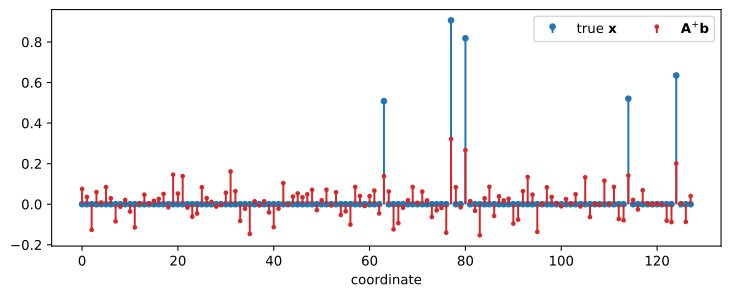
relative error ||x - A^+ b|| / ||x|| = 0.823
sqrt(1 - m/n) = 0.829
||A^+ b||^2 = 0.782,  (m/n)||x||^2 = 0.758
The minimum-norm solution spreads the energy. The annotations: <1> selects the support — five coordinates at random, each with a uniform magnitude in [0.5, 1]; <2> computes the pseudoinverse solution. Two observations deserve comment.
First, the reconstruction is dense: every one of the 128 coordinates carries some mass, and the printed error is 0.82. This is forced. For a Gaussian \mathbf{A} with m < n, the rows are independent with probability one, and then \mathbf{A}^{+}\mathbf{A} = \mathbf{P}_{\mathsf{C}(\mathbf{A}^{\mathsf T})} is the orthogonal projection onto the m-dimensional row space (Chapter 6). The minimum-norm solution is therefore the projection of the true signal onto a random m-dimensional subspace,
\hat{\mathbf{x}} = \mathbf{A}^{+}\mathbf{A}\mathbf{x} = \mathbf{P}_{\mathsf{C}(\mathbf{A}^{\mathsf T})}\mathbf{x},
and a random subspace is aligned with no coordinate in particular: it keeps the expected fraction m/n of the energy, so the relative error is \sqrt{1 - m/n} = 0.829, matching the printed 0.823 and the printed energy identity \lVert\hat{\mathbf{x}}\rVert^2 \approx (m/n)\lVert\mathbf{x}\rVert^2.
This random-projection estimate is the mechanism behind the Johnson–Lindenstrauss lemma. Sharpening it: for a fixed unit vector \mathbf{u}, the chi-square tail bound gives \Pr\big(\big|\,\lVert\mathbf{A}\mathbf{u}\rVert_2^2 - m\big| > \varepsilon m\big) \le 2e^{-c\varepsilon^2 m}, so a single direction keeps its length to within a factor 1 \pm \varepsilon with overwhelmingly high probability, and a covering argument extends this to finitely many directions at once. Problem 3 verifies the expectation empirically.
Second, the failure has nothing to do with noise — \mathbf{b} is exact. It is the recovery rule that fails. The minimum-norm solution is the smallest-energy explanation of the measurements, and the true signal is the opposite of small-energy: it is concentrated on five coordinates. Minimizing energy and finding sparsity are different objectives, and the \ell_2 ball simply has no way to express the second one.
L1 versus L2: the geometry of sparsity
The minimum-norm solution minimizes the \ell_2 norm over the feasible set \{\mathbf{x} : \mathbf{A}\mathbf{x} = \mathbf{b}\}: it is the point of that affine set closest to the origin. The failure above suggests minimizing a different measure of size. For any norm, the solution of \min \lVert\mathbf{x}\rVert over an affine set is the point where the smallest norm ball around the origin touches the set, and the shape of the ball decides the outcome. The \ell_1 unit ball is the diamond with vertices on the coordinate axes — the same unit balls drawn in Chapter 1 — and an affine set touching the smallest \ell_1 ball generically touches it at a vertex, that is, at a point with some coordinates exactly zero. The \ell_2 ball has no vertices, so its touching point is generic: all coordinates nonzero. The figure below puts both balls against the same feasible line.
import numpy as np
import matplotlib.pyplot as plt

t = np.linspace(0, 2 * np.pi, 500)
rho = np.maximum(np.abs(np.cos(t)), np.abs(np.sin(t)))
r1, r2 = 1.5, 3 / np.sqrt(5)                    # smallest L1 radius; L2 radius
ball1 = r1 * np.c_[np.cos(t), np.sin(t)] / rho[:, None]
ball2 = r2 * np.c_[np.cos(t), np.sin(t)]

x1s = np.linspace(-2.2, 3.8, 200)               # feasible line: x1 + 2 x2 = 3
x2s = (3 - x1s) / 2

fig, ax = plt.subplots(1, 2, figsize=(9.5, 4.2))
for a, ball, sol, title in [
    (ax[0], ball1, (0.0, 1.5), 'smallest $\\ell_1$ ball: corner'),
    (ax[1], ball2, (0.6, 1.2), 'smallest $\\ell_2$ ball: tangent'),
]:
    a.plot(ball[:, 0], ball[:, 1], 'C0-', lw=1.5)
    a.plot(x1s, x2s, 'k-', lw=1.2)
    a.plot(*sol, 'C3*', ms=18)
    a.set_xlim(-2.2, 3.8)
    a.set_ylim(-1.8, 3.0)
    a.set_aspect('equal')
    a.set_xlabel('$x_1$')
    a.set_ylabel('$x_2$')
fig.tight_layout()
plt.show()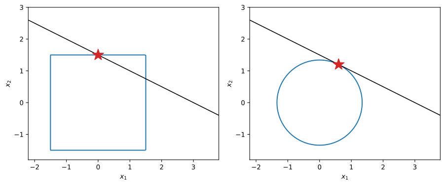
The corner is the sparse point. In the left panel the smallest \ell_1 ball reaching the line touches it at the vertex (0, 1.5), where x_1 = 0; in the right panel the smallest \ell_2 ball touches tangentially at (0.6, 1.2), where both coordinates are nonzero. The pattern generalizes. The \ell_1 ball in \mathbb{R}^n has 2n vertices — the points \pm\mathbf{e}_i on the coordinate axes — so a generic touching point has many exactly-zero coordinates, and the minimum-\ell_1 solution of a generic underdetermined system has at most m nonzero entries: exactly the sparse structure the measurements alone cannot reveal. This is why the recovery rule is basis pursuit: minimize \lVert\mathbf{x}\rVert_1 subject to \mathbf{A}\mathbf{x} = \mathbf{b}. The objective is convex (Chapter 10), so the minimizer is global and reachable by simple iterative algorithms; no combinatorial search over which K coordinates are nonzero is needed. The noisy version of basis pursuit, with the constraint moved into the objective, is the Lasso.
The L1 experiment: Lasso
The model. The Lasso replaces the \ell_2 penalty of ridge regression (Chapter 10) by the \ell_1 penalty,
\boxed{\ \hat{\mathbf{x}} = \operatorname*{arg\,min}_{\mathbf{x}\in\mathbb{R}^n}\ \tfrac{1}{2}\lVert \mathbf{A}\mathbf{x} - \mathbf{b}\rVert_2^2 + \alpha\lVert\mathbf{x}\rVert_1\ }
with \alpha \ge 0 trading fit against sparsity; basis pursuit is the limit \alpha \to 0. Re-running the warm-up on the same \mathbf{A} and \mathbf{b}: tune alpha for the Lasso on a coarse grid, then compare the best Lasso against the Ridge solution.
from sklearn.linear_model import Lasso, Ridge

alphas = [1e-3, 1e-2, 1e-1, 1.0, 10.0]
print('Lasso, tuning alpha:')
print(f'{"alpha":>8} {"rel. error":>10} {"# nonzero":>9} {"support ok":>10}')
for alpha in alphas:
    lasso = Lasso(alpha=alpha, fit_intercept=False, max_iter=20000).fit(A, b)
    x_l1 = lasso.coef_
    supp = np.abs(x_l1) > 1e-4
    ok = np.array_equal(np.sort(np.nonzero(x)[0]), np.sort(np.nonzero(supp)[0]))
    err = np.linalg.norm(x - x_l1) / np.linalg.norm(x)
    print(f'{alpha:8.1e} {err:10.4f} {np.count_nonzero(supp):9d} {str(ok):>10}')

alpha_l1 = 1e-2
x_l1 = Lasso(alpha=alpha_l1, fit_intercept=False, max_iter=20000).fit(A, b).coef_

x_l2 = Ridge(alpha=1e-1, fit_intercept=False).fit(A, b).coef_

fig, ax = plt.subplots(1, 2, figsize=(10, 3.2), sharey=True)
for a, xh, lab, col in [
    (ax[0], x_l1, 'Lasso ($\\ell_1$)', 'C2'),
    (ax[1], x_l2, 'Ridge ($\\ell_2$)', 'C1'),
]:
    s = a.stem(x, linefmt='C0-', markerfmt='C0o', basefmt=' ', label='true $\\mathbf{x}$')
    s.markerline.set_markersize(4)
    s = a.stem(xh, linefmt=col + '-', markerfmt=col + 'o', basefmt=' ', label=lab)
    s.markerline.set_markersize(2.5)
    a.set_xlabel('coordinate')
    a.legend()
ax[0].set_title('Lasso reconstruction')
ax[1].set_title('Ridge reconstruction')
fig.tight_layout()
plt.show()

err_l1 = np.linalg.norm(x - x_l1) / np.linalg.norm(x)
err_l2 = np.linalg.norm(x - x_l2) / np.linalg.norm(x)
print(f'pinv  rel. error = {err_pinv:.3f}')
print(f'ridge rel. error = {err_l2:.3f}')
print(f'lasso rel. error = {err_l1:.3f}  (alpha = {alpha_l1})')
Lasso, tuning alpha:
alpha rel. error # nonzero support ok
1.0e-03 0.0019 5 True
1.0e-02 0.0185 5 True
1.0e-01 0.1847 5 True
1.0e+00 0.9802 1 False
1.0e+01 1.0000 0 False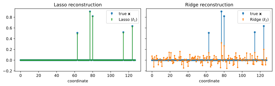
pinv  rel. error = 0.823
ridge rel. error = 0.823
lasso rel. error = 0.018  (alpha = 0.01)
L1 recovers the support, L2 does not. The annotations: <1> fits the Lasso by coordinate descent with no intercept — the model is exactly \mathbf{b} = \mathbf{A}\mathbf{x}; <2> fits the Ridge by a direct linear solve, the same ridge regression as Chapter 10. Three observations.
First, the tuning table: for alpha between 10^{-3} and 10^{-1} the Lasso finds exactly the five true coordinates — the column “support ok” reads True — and the error shrinks as alpha shrinks (1.9\% at \alpha = 10^{-2}). A too-large penalty (\alpha = 1) over-shrinks: every coordinate is crushed toward zero until a single coefficient survives and the support is lost (98\% error). That is the shrinkage bias of \ell_1, not a failure of the geometry.
Second, the left stem plot: the Lasso reconstruction sits on the true support with nearly exact values. The right stem plot: Ridge is dense, with small mass on every coordinate, and its error of 0.82 matches the minimum-norm solution. This is forced: \hat{\mathbf{x}}_{\text{ridge}} = (\mathbf{A}^{\mathsf T}\mathbf{A} + \alpha\mathbf{I})^{-1}\mathbf{A}^{\mathsf T}\mathbf{b} \to \mathbf{A}^{+}\mathbf{b} as \alpha \to 0, so no choice of alpha can make Ridge sparse. The two penalties solve two different problems, and the data are generated by the one the \ell_1 penalty encodes.
How many measurements? The restricted isometry property
The experiment raises a quantitative question: for which pairs (m, K) does \ell_1 recovery work? The answer is a property of the measurement matrix, the restricted isometry property (RIP): \mathbf{A} acts like an isometry on the set of K-sparse vectors. Concretely, \mathbf{A} has RIP constant \delta_K if
(1 - \delta_K)\lVert\mathbf{x}\rVert_2^2 \le \lVert\mathbf{A}\mathbf{x}\rVert_2^2 \le (1 + \delta_K)\lVert\mathbf{x}\rVert_2^2 \qquad \text{for every } K\text{-sparse } \mathbf{x}.
If \delta_{2K} is small — the standard sufficient condition is \delta_{2K} < \sqrt{2} - 1 — then the minimum-\ell_1 solution of \mathbf{A}\mathbf{x} = \mathbf{b} recovers every K-sparse signal exactly. The intuition: a small \delta_{2K} means no K-sparse vector lies near the null space of \mathbf{A}, so the measurements separate all K-sparse candidates, and the \ell_1 minimizer is the sparsest one consistent with \mathbf{b}. The proof is a convexity argument comparing the \ell_1 and \ell_2 norms on 2K-sparse vectors, not reproduced here.1
The RIP is a property of random matrices. A Gaussian \mathbf{A} with
\boxed{\ m \gtrsim K\log(n/K)\ }
rows satisfies the RIP with \delta_{2K} < \sqrt{2} - 1 with high probability, and the constant hidden in \gtrsim is an absolute constant independent of n and K.2 The logarithmic factor is the price of not knowing the support in advance: choosing K of n coordinates is a combinatorial decision carrying about \log\binom{n}{K} \approx K\log(n/K) bits of information, and each measurement must contribute a comparable amount. The warm-up is consistent with the bound: K\log(n/K) = 5\log(128/5) \approx 16, and m = 40 measurements sufficed comfortably.
The same convexity that guarantees a global minimizer (Chapter 10) guarantees tractability: the \ell_1 objective is convex, so recovery is a convex optimization problem solvable by simple first-order iterations, with no combinatorial search over supports.
A CT-style phantom
The one-dimensional experiment transfers directly to imaging. The model. The ground truth is a 48\times 48 image of six bright disks on a black canvas — a sparse image in the pixel basis, in the spirit of the Shepp–Logan phantom used to benchmark tomography algorithms. The next cell draws it.
The measurements. An X-ray projection at angle \theta is the set of line integrals of the image along parallel rays: rotate the image by \theta and sum along the rows. Each projection contributes 48 measurements (one per row), and a measurement matrix \mathbf{A} carries one row per ray. With 16 angles spanning 0^\circ to 165^\circ in steps of 11^\circ, the system has m = 16 \times 48 = 768 rows and n = 2304 columns: about a third of the pixels are “measured”, yet the image is only about 9% nonzero, so the RIP heuristic of the previous section says recovery is feasible.
side = 48
yy, xx = np.mgrid[0:side, 0:side].astype(float)

def disk(cx, cy, r, v):
    """Filled disk: intensity v, radius r, center (cx, cy)."""
    return v * ((xx - cx) ** 2 + (yy - cy) ** 2 <= r ** 2)

x_2d = np.zeros((side, side))
for (cx, cy, r, v) in [(18, 18, 4, 1.0), (30, 16, 3, 0.8), (24, 28, 4, 0.9),
                       (14, 30, 3, 0.7), (34, 30, 3, 0.6), (22, 38, 3, 0.8)]:
    x_2d += disk(cx, cy, r, v)
x_2d = np.clip(x_2d, 0.0, 1.0)

K2 = np.count_nonzero(x_2d)
fig, ax = plt.subplots(figsize=(4, 4))
ax.imshow(x_2d, cmap='gray_r', origin='lower')
ax.set_xticks([])
ax.set_yticks([])
plt.show()

print(f'image: {side} x {side} = {side * side} pixels,'
      f'  {K2} nonzero ({100 * K2 / side ** 2:.1f}%)')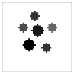
image: 48 x 48 = 2304 pixels, 214 nonzero (9.3%)The measurement operator. One projection: rotate the image by \theta and sum the rows with scipy.ndimage.rotate (bilinear interpolation, same canvas), then sum(axis=1). The matrix \mathbf{A} applies this operator to every pixel: column j of \mathbf{A} is the projection of the j-th basis image (a single pixel of value 1). Rather than rotating 2304 images one by one, the cell stacks them into one array of shape (2304, 48, 48) and rotates the stack once per angle — ndimage.rotate with axes=(1, 2) rotates every plane independently, so the planes never mix.
import scipy.ndimage as ndi

angles = np.linspace(0, 165, 16)
n_angles = len(angles)
n_pix = side * side
m = n_angles * side

basis = np.zeros((n_pix, side, side))
idx = np.arange(n_pix)
basis[idx, idx // side, idx % side] = 1.0

A_2d = np.empty((m, n_pix))
for k, theta in enumerate(angles):
    rot = ndi.rotate(basis, theta, axes=(1, 2), reshape=False, order=1)
    A_2d[k * side:(k + 1) * side] = rot.sum(axis=1).T

b_2d = A_2d @ x_2d.ravel()
print(f'A: {m} x {n_pix},  sampling ratio m/n = {m / n_pix:.2f}')
A: 768 x 2304, sampling ratio m/n = 0.33The matrix. The annotations: <1> the 16 projection angles, 0^\circ to 165^\circ in steps of 11^\circ; <2> the stack of basis images, one per pixel; <3> rotates every plane of the stack by the same angle in a single call; <4> sums the rows of each rotated basis image and writes the result into the block of \mathbf{A} for angle k.
The resulting operator is 768 \times 2304: the measurements \mathbf{b} = \mathbf{A}\mathbf{x} use a third of the pixel count. The phantom has K = 214 nonzero pixels, and the heuristic of the previous section gives K\log(n/K) = 214\log(2304/214) \approx 508 < 768: the measurement budget is sufficient, with room to spare. The next cell runs both recovery rules on the same \mathbf{b}.
Reconstruction: L2 smears, L1 concentrates
The comparison. Both solvers see the same measurements \mathbf{b}. Ridge at alpha = 1e-1 represents the \ell_2 route — its error is flat across a wide range of alpha, since the ridge solution is pinned to the minimum-norm solution; Lasso at alpha = 1e-3 represents the \ell_1 route, chosen from the same small grid used for the one-dimensional experiment. The figure below shows the phantom, the Ridge reconstruction, and the Lasso reconstruction; the printed errors are relative residuals \lVert\mathbf{x} - \hat{\mathbf{x}}\rVert_2 / \lVert\mathbf{x}\rVert_2.
from sklearn.linear_model import Ridge, Lasso

print('relative errors ||x - x_hat|| / ||x||:')
for alpha in [1e-3, 1e-2, 1e-1]:
    x_l = Lasso(alpha=alpha, fit_intercept=False, max_iter=20000).fit(A_2d, b_2d).coef_
    print(f'  Lasso  alpha={alpha:8.1e}  {np.linalg.norm(x_2d.ravel() - x_l) / np.linalg.norm(x_2d):.4f}')
for alpha in [1e-1, 1.0, 10.0]:
    x_r = Ridge(alpha=alpha, fit_intercept=False).fit(A_2d, b_2d).coef_
    print(f'  Ridge  alpha={alpha:8.1e}  {np.linalg.norm(x_2d.ravel() - x_r) / np.linalg.norm(x_2d):.4f}')

x_ridge = Ridge(alpha=1e-1, fit_intercept=False).fit(A_2d, b_2d).coef_.reshape(side, side)
x_lasso = Lasso(alpha=1e-3, fit_intercept=False, max_iter=20000).fit(A_2d, b_2d).coef_.reshape(side, side)

fig, ax = plt.subplots(1, 3, figsize=(11, 3.8))
for a, im, t in zip(ax, [x_2d, x_ridge, x_lasso],
                    ['phantom', 'Ridge ($\\ell_2$)', 'Lasso ($\\ell_1$)']):
    a.imshow(im, cmap='gray_r', origin='lower')
    a.set_title(t)
    a.set_xticks([])
    a.set_yticks([])
fig.tight_layout()
plt.show()

err_r = np.linalg.norm(x_2d.ravel() - x_ridge.ravel()) / np.linalg.norm(x_2d)
err_l = np.linalg.norm(x_2d.ravel() - x_lasso.ravel()) / np.linalg.norm(x_2d)
print(f'ridge rel. error = {err_r:.3f}')
print(f'lasso rel. error = {err_l:.3f}')
relative errors ||x - x_hat|| / ||x||:
Lasso alpha= 1.0e-03 0.0438
Lasso alpha= 1.0e-02 0.3991
Lasso alpha= 1.0e-01 0.7959
Ridge alpha= 1.0e-01 0.3391
Ridge alpha= 1.0e+00 0.3421
Ridge alpha= 1.0e+01 0.3723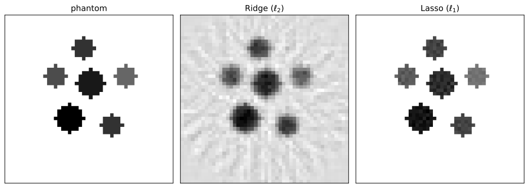
ridge rel. error = 0.339
lasso rel. error = 0.044
L2 smears, L1 concentrates. The annotations: <1> the Ridge reconstruction, <2> the Lasso reconstruction at the tuned alpha. Two observations.
First, Ridge fails in exactly the way the one-dimensional experiment predicted. Its solution is dense — every pixel carries some faint intensity — so each disk appears as a soft halo spread over the whole canvas, and the relative error is 0.34. The image content is “explained” by energy that is everywhere, which is the \ell_2 ball doing what its geometry forces. Second, Lasso recovers the phantom structure: the six disks reappear at the right positions with the right intensities, at a relative error of 0.04, with mild speckle artifacts and slightly shrunken intensities — the \ell_1 bias seen in the tuning table.
The solver is worth a closing remark. Coordinate descent, the algorithm behind Lasso, is linear algebra under the hood: each step is a matrix-vector product with \mathbf{A} and \mathbf{A}^{\mathsf T}, plus one nonlinear entrywise step — the soft-thresholding operator of Chapter 13. The nonlinearity is exactly where sparsity enters; everything else is the machinery of Chapters 3, 6, and 8.
L1 versus L2 at a glance
| \ell_1 (Lasso, basis pursuit) | \ell_2 (Ridge, min-norm) | |
|---|---|---|
| Penalty | \alpha\lVert\mathbf{x}\rVert_1 | \alpha\lVert\mathbf{x}\rVert_2^2 |
| Penalty ball | corners on the coordinate axes | round, no corners |
| Typical solution | few nonzero entries | all entries nonzero |
| Underdetermined systems | recovers a sparse support | spreads energy, dense |
| Failure mode | bias and support instability under heavy noise | misses sparsity entirely |
| Right when | signal genuinely sparse, m \ll n | dense signal, m \ge n |
Note
The measurement budget. The working heuristic for sparse recovery: m \gtrsim K\log(n/K), where K is the number of nonzero entries of \mathbf{x}. The precise guarantee (Candès–Romberg–Tao 2006; Donoho 2006) is that a random Gaussian \mathbf{A} with m \ge CK\log(n/K) rows satisfies the restricted isometry property with high probability, and that the minimum-\ell_1 solution then recovers every K-sparse signal exactly — stably, in the presence of noise. In practice the constant C is a small number (roughly 2–4), so the heuristic is a genuine guide, not just an asymptotic statement.
The applications are wherever acquisition is the bottleneck: computed tomography with fewer projections (less radiation), MRI with fewer k-space samples (shorter scans), radar, astronomy, and sensor networks. In each case the hardware measures linear combinations of the signal; compressed sensing says the recovery algorithm — not the scanner — decides how many are needed. See the Wikipedia articles on compressed sensing, basis pursuit, and the Lasso.
Summary
- Underdetermined plus sparse means \ell_1. The minimum-norm solution \mathbf{A}^{+}\mathbf{b} minimizes energy, not sparsity, and on a 5-sparse signal in \mathbb{R}^{128} its relative error is \sqrt{1 - m/n} = 0.83: the reconstruction is dense because a random row space aligns with no coordinate. The Lasso with \alpha = 10^{-2} recovers the support exactly, at 1.9\% error.
- The geometry decides. The \ell_1 ball has corners on the coordinate axes, so the smallest ball touching the feasible set touches at a corner — a sparse point. The \ell_2 ball is round, so its touching point is dense. The same geometry reappears in two dimensions: Ridge smears the phantom (34% error), Lasso recovers it (4% error).
- The count. A Gaussian measurement matrix satisfies the restricted isometry property with high probability once m \gtrsim K\log(n/K); under the RIP the \ell_1 minimizer recovers every K-sparse signal exactly, and convexity (Chapter 10) keeps the search tractable.
This closes the applications arc of the course: Chapter 11 put the SVD/NMF decomposition to work on topic modeling, Chapter 12 the eigenvector machinery on PageRank, Chapter 13 the low-rank-plus-sparse decomposition on robust PCA, and this chapter the sparse-recovery geometry on compressed sensing. Four problems, one arc: each is a decomposition or optimization idea from the first ten chapters, applied where the data are large and the structure is small.
Problems
The problems below exercise the compressed-sensing machinery: the energy identity behind the minimum-norm failure (14-1, 14-3), the sparsity of the minimum-\ell_1 solution (14-2), the restricted isometry property (14-4), and the phase transition in the measurement count (14-5). All random draws use fixed seeds, so every numerical outcome is reproducible.
[P14.1] The energy identity for the minimum-norm solution
The minimum-norm solution \hat{\mathbf{x}} = \mathbf{A}^{+}\mathbf{b} is the projection of the true signal onto the row space of \mathbf{A}. This problem derives the expected energy of that projection.
Let \mathbf{A} \in \mathbb{R}^{m \times n} be Gaussian with m < n. Show that \mathbf{P} = \mathbf{A}^{+}\mathbf{A} is the orthogonal projection onto \mathsf{C}(\mathbf{A}^{\mathsf T}), and write \mathbf{P} = \sum_{i=1}^{m} \mathbf{u}_i \mathbf{u}_i^{\mathsf T} for an orthonormal basis \{\mathbf{u}_i\} of the row space.
By rotational invariance of the Gaussian distribution, show that \mathbb{E}[\mathbf{u}_i \mathbf{u}_i^{\mathsf T}] = \tfrac{1}{n}\mathbf{I} for each i.
Conclude that for any fixed \mathbf{x},
\boxed{\ \mathbb{E}\lVert \mathbf{P}\mathbf{x}\rVert_2^2 = \frac{m}{n}\lVert \mathbf{x}\rVert_2^2\ },
and hence the expected relative error of the minimum-norm solution is \sqrt{1 - m/n}.
[P14.2] Sparsity of the minimum-\ell_1 solution
Basis pursuit minimizes \lVert \mathbf{x}\rVert_1 over the affine set \{\mathbf{x} : \mathbf{A}\mathbf{x} = \mathbf{b}\}. This problem shows that the solution is sparse.
- Let \mathbf{A} \in \mathbb{R}^{m \times n} have full row rank. Write the problem as a standard-form linear program in the variables \mathbf{x}^{+}, \mathbf{x}^{-} \in \mathbb{R}^n with \mathbf{x} = \mathbf{x}^{+} - \mathbf{x}^{-} and \mathbf{x}^{+}, \mathbf{x}^{-} \ge 0:
\min_{\mathbf{x}^{+}, \mathbf{x}^{-}} \ \mathbf{1}^{\mathsf T}\mathbf{x}^{+} + \mathbf{1}^{\mathsf T}\mathbf{x}^{-} \quad \text{subject to} \quad \mathbf{A}\mathbf{x}^{+} - \mathbf{A}\mathbf{x}^{-} = \mathbf{b}, \quad \mathbf{x}^{+}, \mathbf{x}^{-} \ge 0.
Argue that the optimum is attained at a vertex of the feasible polytope, and that a vertex has at most m nonzero coordinates. (A basic feasible solution of a standard-form LP with m equality constraints has at most m nonzero variables.)
Conclude that the minimum-\ell_1 solution has at most m nonzero entries. Why does this make basis pursuit a plausible recovery rule for K-sparse signals with m \ge K measurements?
[P14.3] Verifying the energy identity numerically
The energy identity of Problem 14-1 predicts that the minimum-norm solution keeps the fraction m/n of the signal energy. The starter code draws a Gaussian \mathbf{A} \in \mathbb{R}^{40 \times 128}, forms \mathbf{P} = \mathbf{A}^{+}\mathbf{A}, and measures \lVert \mathbf{P}\mathbf{x}\rVert_2^2 over T = 2000 random unit-norm signals.
Verify that the empirical mean of \lVert \mathbf{P}\mathbf{x}\rVert_2^2 matches m/n = 0.3125.
Verify that \sqrt{1 - \text{mean}} matches the predicted relative error \sqrt{1 - m/n} \approx 0.829.
The starter code prints both comparisons.
import numpy as np

rng = np.random.default_rng(3)
n, m, T = 128, 40, 2000
A = rng.standard_normal((m, n))
P = np.linalg.pinv(A) @ A

xs = rng.standard_normal((T, n))
xs = xs / np.linalg.norm(xs, axis=1, keepdims=True)
energies = np.sum((xs @ P.T) ** 2, axis=1)

print("mean ||P x||^2 =", energies.mean(), "  m/n =", m / n)
print("sqrt(1 - mean) =", np.sqrt(1 - energies.mean()), "  sqrt(1 - m/n) =", np.sqrt(1 - m / n))
mean ||P x||^2 = 0.3122261693238835 m/n = 0.3125
sqrt(1 - mean) = 0.8293213072604106 sqrt(1 - m/n) = 0.82915619758885[P14.4] Estimating the restricted isometry constant
The restricted isometry constant \delta_K of a matrix \mathbf{A} is the worst-case deviation of \lVert \mathbf{A}\mathbf{x}\rVert_2^2 from \lVert \mathbf{x}\rVert_2^2 over K-sparse \mathbf{x}. For a scaled Gaussian matrix, entries \mathcal{N}(0, 1/m), the constant is small when m \gg K\log(n/K). The starter code estimates \delta_5 by sampling T = 2000 random 5-sparse unit vectors for three measurement counts.
Report the three estimates and verify that they decrease with m: more measurements, better isometry.
Verify the scaling \delta_5 \cdot \sqrt{m} is roughly constant across the three values, consistent with a deviation that decays like 1/\sqrt{m}.
The starter code prints the estimates.
import numpy as np

rng = np.random.default_rng(5)
n, K, T = 128, 5, 2000

def est_delta(m):
    """Estimate delta_K by sampling random K-sparse unit vectors."""
    A = rng.standard_normal((m, n)) / np.sqrt(m)
    vals = []
    for _ in range(T):
        x = np.zeros(n)
        x[rng.choice(n, K, replace=False)] = rng.standard_normal(K)
        x = x / np.linalg.norm(x)
        vals.append(np.linalg.norm(A @ x) ** 2)
    return max(vals) - 1.0

for m in (40, 80, 160):
    d = est_delta(m)
    print(f"m={m}: delta_5 ~ {d:.4f},  delta_5 * sqrt(m) = {d * np.sqrt(m):.3f}")
m=40: delta_5 ~ 1.0322, delta_5 * sqrt(m) = 6.528
m=80: delta_5 ~ 0.5780, delta_5 * sqrt(m) = 5.170
m=160: delta_5 ~ 0.4935, delta_5 * sqrt(m) = 6.242[P14.5] The phase transition in the number of measurements
Challenge. The heuristic m \gtrsim K\log(n/K) predicts how many measurements suffice for exact recovery. This experiment measures the transition empirically.
For n = 128, K = 5, and each m \in \{8, 12, 16, 20, 24, 28, 32, 40\}, run T = 20 trials: draw a K-sparse signal \mathbf{x}, a Gaussian \mathbf{A} \in \mathbb{R}^{m \times n}, and measurements \mathbf{b} = \mathbf{A}\mathbf{x}; recover with basis pursuit, the \alpha \to 0 limit of the Lasso; declare success when the recovered support matches the true support exactly. Record the success fraction.
Plot the success fraction against m and overlay the heuristic K\log(n/K) \approx 16.2.
Report the smallest m with success fraction 1.0 and compare it with the heuristic.
The starter code defines the basis-pursuit solver and runs the trials.
import numpy as np
from scipy.optimize import linprog

def bp_solve(A, b):
    """Basis pursuit: min ||x||_1 s.t. Ax = b, via LP."""
    m, n = A.shape
    c = np.ones(2 * n)
    Aeq = np.hstack([A, -A])
    res = linprog(c, A_eq=Aeq, b_eq=b, bounds=(0, None), method="highs")
    return res.x[:n] - res.x[n:]

n, K, T = 128, 5, 20
ms = [8, 12, 16, 20, 24, 28, 32, 40]

for m in ms:
    rng = np.random.default_rng(100 + m)
    succ = 0
    for t in range(T):
        x = np.zeros(n)
        x[rng.choice(n, K, replace=False)] = rng.uniform(0.5, 1.0, K)
        A = rng.standard_normal((m, n))
        b = A @ x
        xh = bp_solve(A, b)
        supp = np.abs(xh) > 1e-4
        if np.array_equal(np.sort(np.nonzero(x)[0]), np.sort(np.nonzero(supp)[0])):
            succ += 1
    print(f"m={m:3d}: success {succ}/{T}")
m= 8: success 0/20
m= 12: success 1/20
m= 16: success 4/20
m= 20: success 6/20
m= 24: success 16/20
m= 28: success 20/20
m= 32: success 20/20
m= 40: success 20/20Footnotes
Precise statement: a Gaussian \mathbf{A}\in\mathbb{R}^{m\times n} satisfies the RIP with constant \delta_{2K} with probability 1 - e^{-ct} once m \ge CK\log(n/K) + t. The exact-recovery guarantee is due to Candès, Romberg, and Tao (2006) and, independently, Donoho (2006); see the Wikipedia article on the restricted isometry property.↩︎
Precise statement: a Gaussian \mathbf{A}\in\mathbb{R}^{m\times n} satisfies the RIP with constant \delta_{2K} with probability 1 - e^{-ct} once m \ge CK\log(n/K) + t. The exact-recovery guarantee is due to Candès, Romberg, and Tao (2006) and, independently, Donoho (2006); see the Wikipedia article on the restricted isometry property.↩︎