from watchtower.core import set_format
set_format("svg")PageRank
The World Wide Web is a directed graph: pages are nodes and hyperlinks are edges, pointing from the page that contains them to the page they reference. Ranking pages by importance is the problem that founded the search industry, and its solution rests on one recursive idea: a page is important if important pages link to it. The definition is circular, which is precisely what makes it a fixed-point problem: the kind this course has a tool for.
Chapter 9 ended with the power method, the iterative engine that finds a matrix’s dominant eigenvector using nothing but matrix-vector products, and noted in passing that it is the algorithm behind PageRank. This chapter makes good on that claim. The link structure becomes a matrix, importance becomes an eigenvector, and the power method becomes the ranking algorithm. Two ingredients appear that Chapter 9’s symmetric demo did not exercise: the matrix is nonsymmetric and column-stochastic: the transition matrix of a Markov chain.
The view that makes the connection work is the random surfer: a hypothetical reader who starts on a random page, follows a random link on each page, and repeats forever. The fraction of time the surfer spends on each page is a natural measure of importance, and the graph alone determines it — again a fixed point, this time of a probabilistic system.
A teaching web
The ideas are developed on a small synthetic web of sixteen pages, labeled \mathrm{A} through \mathrm{P}, engineered to contain the three structures that break naive ranking: two hubs (pages with many out-links), a dangling node (a page with no out-links at all), and a sink cluster (a group of pages that link only to one another). The link structure is deliberately asymmetric: page \mathrm{A} receives eleven in-links while page \mathrm{P} receives none, so a sensible ranking is not obvious from link counts alone.
The adjacency matrix \mathbf{A} \in \mathbb{R}^{n \times n} records the links: A_{ds} = 1 when page s links to page d, and 0 otherwise. Column s lists the out-links of page s; row d lists the in-links of page d.
| Page | Out-links | Page | Out-links |
|---|---|---|---|
| A | B C D E F G H | I | J K |
| B | A C D | J | I K |
| C | A B | K | I J |
| D | A B | L | A B C |
| E | A | M | A L |
| F | A B | N | A M |
| G | A B | O | A N |
| H | none | P | A O |
Column \mathrm{H} is empty: the dangling node. And because \mathrm{I}, \mathrm{J}, \mathrm{K} link only to one another, no surfer mass that enters that cluster can ever leave it, a fact that will matter shortly.
import numpy as np
import networkx as nx
import matplotlib.pyplot as plt

pages = list('ABCDEFGHIJKLMNOP')
out = {'A': 'BCDEFGH', 'B': 'ACD', 'C': 'AB', 'D': 'AB', 'E': 'A',
       'F': 'AB', 'G': 'AB', 'H': '', 'I': 'JK', 'J': 'IK', 'K': 'IJ',
       'L': 'ABC', 'M': 'AL', 'N': 'AM', 'O': 'AN', 'P': 'AO'}

n = len(pages)
index = {p: i for i, p in enumerate(pages)}
A = np.zeros((n, n))
for s, dests in out.items():
    for d in dests:
        A[index[d], index[s]] = 1.0

G = nx.DiGraph()
G.add_nodes_from(pages)
G.add_edges_from((s, d) for s, dests in out.items() for d in dests)

colors = {'A': 'tab:red', 'B': 'tab:orange', 'H': 'tab:gray',
          'I': 'tab:blue', 'J': 'tab:blue', 'K': 'tab:blue'}
node_color = [colors.get(p, 'lightsteelblue') for p in pages]
pos = nx.spring_layout(G, seed=0, k=1.2, iterations=60)

fig, ax = plt.subplots(figsize=(7.5, 6.5))
nx.draw_networkx(G, pos, ax=ax, node_color=node_color, node_size=900,
                 font_size=13, arrowsize=14, edge_color='gray', width=1.2)
for label, c in [('hub A', 'tab:red'), ('hub B', 'tab:orange'),
                 ('dangling H', 'tab:gray'), ('sink cluster', 'tab:blue'),
                 ('leaf', 'lightsteelblue')]:
    ax.scatter([], [], c=c, s=90, label=label)
ax.legend(loc='lower left', frameon=False)
ax.axis('off')
fig.tight_layout()
plt.show()

print(A.astype(int))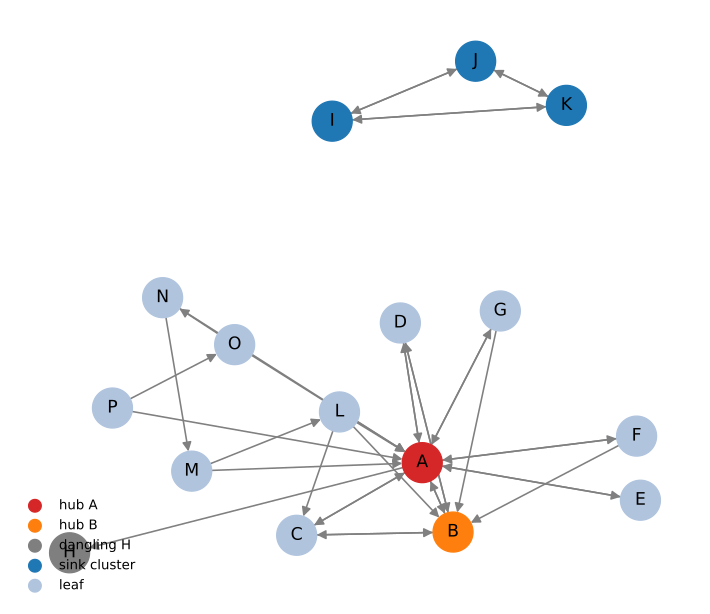
[[0 1 1 1 1 1 1 0 0 0 0 1 1 1 1 1]
 [1 0 1 1 0 1 1 0 0 0 0 1 0 0 0 0]
 [1 1 0 0 0 0 0 0 0 0 0 1 0 0 0 0]
 [1 1 0 0 0 0 0 0 0 0 0 0 0 0 0 0]
 [1 0 0 0 0 0 0 0 0 0 0 0 0 0 0 0]
 [1 0 0 0 0 0 0 0 0 0 0 0 0 0 0 0]
 [1 0 0 0 0 0 0 0 0 0 0 0 0 0 0 0]
 [1 0 0 0 0 0 0 0 0 0 0 0 0 0 0 0]
 [0 0 0 0 0 0 0 0 0 1 1 0 0 0 0 0]
 [0 0 0 0 0 0 0 0 1 0 1 0 0 0 0 0]
 [0 0 0 0 0 0 0 0 1 1 0 0 0 0 0 0]
 [0 0 0 0 0 0 0 0 0 0 0 0 1 0 0 0]
 [0 0 0 0 0 0 0 0 0 0 0 0 0 1 0 0]
 [0 0 0 0 0 0 0 0 0 0 0 0 0 0 1 0]
 [0 0 0 0 0 0 0 0 0 0 0 0 0 0 0 1]
 [0 0 0 0 0 0 0 0 0 0 0 0 0 0 0 0]]
The teaching graph.
<1>The adjacency convention: a 1 in row d, column s says page s links to page d, so column s is the out-link list of page s.<2>Empty scatter points supply the legend: hubs in red and orange, the dangling node in gray, the sink cluster in blue, leaves in light blue.
The printed matrix makes the structure legible. Column \mathrm{H} is entirely zero: the dangling node. The submatrix on rows and columns \mathrm{I}, \mathrm{J}, \mathrm{K} is the closed cluster: its columns have their 1s inside the cluster and nowhere else, so mass that enters it never leaves. Page \mathrm{A}’s row holds eleven 1s, the most in-links of any page; page \mathrm{P}’s row is empty. A naive “count the in-links” ranking would put \mathrm{A} first and \mathrm{P} last, which is the right spirit, but the closed cluster will defeat the naive linear ranking below.
From links to probabilities
A surfer at page s picks uniformly among its out-links. Normalizing column s of \mathbf{A} by the out-degree \operatorname{out}(s) = \sum_d A_{ds} turns each column into a probability distribution over the next page:
\mathbf{P}_{ds} = \frac{A_{ds}}{\operatorname{out}(s)}, \qquad \sum_d \mathbf{P}_{ds} = 1.
The matrix \mathbf{P} is column-stochastic: nonnegative entries with every column summing to one. It is the transition matrix of a Markov chain on the pages: \mathbf{P}_{ds} is the probability that a surfer at page s moves to page d. Unlike every matrix iterated in Chapter 9, \mathbf{P} is not symmetric: the web’s links point one way, so the full nonsymmetric machinery of that chapter applies.
The cell below builds \mathbf{P} and records its spectrum. The dangling column \mathrm{H} is left as a zero column for now; the division by \operatorname{out}(\mathrm{H}) = 0 is undefined, and confronting that undefinedness is the point.
import numpy as np

outdeg = A.sum(axis=0)
with np.errstate(divide='ignore', invalid='ignore'):
    P = A / outdeg
P = np.nan_to_num(P, nan=0.0)

print('out-degrees :', dict(zip(pages, outdeg.astype(int).tolist())))
print('column sums :', np.round(P.sum(axis=0), 3))
print()
print('P =')
print(np.round(P, 2))

lam = np.linalg.eigvals(P)
lam_abs = np.sort(np.abs(lam))[::-1]
print()
print('|lambda_1|         =', np.round(lam_abs[0], 6))
print('|lambda_2/lambda_1| =', np.round(lam_abs[1] / lam_abs[0], 6))
out-degrees : {'A': 7, 'B': 3, 'C': 2, 'D': 2, 'E': 1, 'F': 2, 'G': 2, 'H': 0, 'I': 2, 'J': 2, 'K': 2, 'L': 3, 'M': 2, 'N': 2, 'O': 2, 'P': 2}
column sums : [1. 1. 1. 1. 1. 1. 1. 0. 1. 1. 1. 1. 1. 1. 1. 1.]
P =
[[0. 0.33 0.5 0.5 1. 0.5 0.5 0. 0. 0. 0. 0.33 0.5 0.5
0.5 0.5 ]
[0.14 0. 0.5 0.5 0. 0.5 0.5 0. 0. 0. 0. 0.33 0. 0.
0. 0. ]
[0.14 0.33 0. 0. 0. 0. 0. 0. 0. 0. 0. 0.33 0. 0.
0. 0. ]
[0.14 0.33 0. 0. 0. 0. 0. 0. 0. 0. 0. 0. 0. 0.
0. 0. ]
[0.14 0. 0. 0. 0. 0. 0. 0. 0. 0. 0. 0. 0. 0.
0. 0. ]
[0.14 0. 0. 0. 0. 0. 0. 0. 0. 0. 0. 0. 0. 0.
0. 0. ]
[0.14 0. 0. 0. 0. 0. 0. 0. 0. 0. 0. 0. 0. 0.
0. 0. ]
[0.14 0. 0. 0. 0. 0. 0. 0. 0. 0. 0. 0. 0. 0.
0. 0. ]
[0. 0. 0. 0. 0. 0. 0. 0. 0. 0.5 0.5 0. 0. 0.
0. 0. ]
[0. 0. 0. 0. 0. 0. 0. 0. 0.5 0. 0.5 0. 0. 0.
0. 0. ]
[0. 0. 0. 0. 0. 0. 0. 0. 0.5 0.5 0. 0. 0. 0.
0. 0. ]
[0. 0. 0. 0. 0. 0. 0. 0. 0. 0. 0. 0. 0.5 0.
0. 0. ]
[0. 0. 0. 0. 0. 0. 0. 0. 0. 0. 0. 0. 0. 0.5
0. 0. ]
[0. 0. 0. 0. 0. 0. 0. 0. 0. 0. 0. 0. 0. 0.
0.5 0. ]
[0. 0. 0. 0. 0. 0. 0. 0. 0. 0. 0. 0. 0. 0.
0. 0.5 ]
[0. 0. 0. 0. 0. 0. 0. 0. 0. 0. 0. 0. 0. 0.
0. 0. ]]
|lambda_1| = 1.0
|lambda_2/lambda_1| = 0.952378The stochastic matrix.
<1>The out-degree of page s is the sum of column s of \mathbf{A}.<2>The dangling column \mathrm{H} produced a 0/0; it is set to zero rather than left asnan.
Every nonzero column of \mathbf{P} sums to one, as the printed column sums show; the exception is column \mathrm{H}, whose out-degree is zero. The spectrum already shows \lambda_1 = 1: the closed cluster \{\mathrm{I}, \mathrm{J}, \mathrm{K}\} never links out, so its own submatrix is column-stochastic and its dominant eigenvalue survives inside \mathbf{P}. And |\lambda_2/\lambda_1| = 0.952, so by the convergence-rate formula of Chapter 9 the power method will need hundreds of iterations here, a first hint that the undamped matrix is not through misbehaving.
Column-stochasticity is a statement about the left eigenvector: \mathbf{1}^{\mathsf T}\mathbf{P} = \mathbf{1}^{\mathsf T}. The ranking lives on the right side: a vector \mathbf{x} with \mathbf{P}\mathbf{x} = \mathbf{x}, \mathbf{x} \ge \mathbf{0} and \sum_d x_d = 1 is a stationary distribution, the long-run fraction of visits the surfer pays to each page. For the symmetric matrices of Chapters 2 and 9 the two sides coincide; for a nonsymmetric \mathbf{P} they are different objects, and the biorthogonality of Chapter 9 becomes operational.
Power iteration, undamped
Chapter 9’s power method finds the dominant eigenvector by iterating \mathbf{x}_{k+1} = \mathbf{P}\mathbf{x}_k and renormalizing. Nothing in its derivation required symmetry, so it applies to the nonsymmetric \mathbf{P} unchanged; only the normalization differs. Chapter 9 normalized to unit 2-norm to feed the Rayleigh quotient; here the limit is a probability distribution, so the iterates are normalized to sum to one. The two normalizations change the scale, not the direction, and the direction is what converges.
The convergence rate is the same formula as in Chapter 9: the error in direction decays like |\lambda_2/\lambda_1|^k, now 0.952^k. The iteration below runs until consecutive iterates agree to 10^{-10} in the 2-norm.
def power_method(P, max_iter=5000, tol=1e-10):
    """Dominant right eigenvector of P: x_{k+1} = P x_k, normalized to sum one."""
    n = P.shape[0]
    x = np.full(n, 1.0 / n)
    residuals = []
    for k in range(max_iter):
        x_new = P @ x
        x_new = x_new / x_new.sum()
        residuals.append(np.linalg.norm(x_new - x, 2))
        if residuals[-1] < tol:
            break
        x = x_new
    return x, np.array(residuals), k + 1

scores, residuals, iters = power_method(P)
rank = np.argsort(-scores)

print(f'converged in {iters} iterations, final residual {residuals[-1]:.1e}')
for i in rank:
    print(f'  {pages[i]}: {scores[i]:.6f}')
converged in 434 iterations, final residual 1.0e-10
I: 0.333333
J: 0.333333
K: 0.333333
A: 0.000000
B: 0.000000
C: 0.000000
D: 0.000000
E: 0.000000
F: 0.000000
G: 0.000000
H: 0.000000
L: 0.000000
M: 0.000000
N: 0.000000
O: 0.000000
P: 0.000000The undamped ranking.
<1>One matrix-vector product per step; this is the entire per-iteration cost of the method, as in Chapter 9.<2>Sum-to-one normalization keeps \mathbf{x} a probability vector; only the direction matters for convergence.
The iteration converged and produced a ranking that is obviously wrong. All of the probability mass sits on the sink cluster \{\mathrm{I}, \mathrm{J}, \mathrm{K}\}, split evenly, and every other page — including \mathrm{A}, the most-linked page in the graph — scores zero to six decimals. The failure has two independent causes, each a violation of an assumption the eigenvector story silently makes.
| Failure | Mechanism |
|---|---|
| Dangling node \mathrm{H} | Column \mathrm{H} of \mathbf{P} is zero, so a surfer at \mathrm{H} has no next page. Mass vanishes at \mathrm{H} instead of circulating, and the matrix is not stochastic. |
| Closed sink cluster | \{\mathrm{I}, \mathrm{J}, \mathrm{K}\} is a reducible component: mass that enters can never leave. The stationary distribution here is still unique — the sink is the only closed class — but it lives entirely on those three pages, so importance becomes local and every page outside scores zero. (With a second closed class even uniqueness would fail.) |
Both defects are repaired by a single mechanism: damping.
Damping and the Google matrix
The two failures share a root cause: the surfer can get trapped, at \mathrm{H} with nowhere to go, or inside a cluster with no way out. The PageRank remedy makes getting trapped impossible, in two small edits to \mathbf{P}.
Dangling repair. A surfer at a page with no out-links picks a uniformly random page. Replace every zero column of \mathbf{P} by the uniform column \tfrac{1}{n}\mathbf{1}; call the result \widetilde{\mathbf{P}}, which is now genuinely column-stochastic.
Teleportation. At every step the surfer follows a link with probability \alpha and jumps to a uniformly random page with probability 1-\alpha. The transition matrix of this modified walk is the Google matrix
\boxed{\;\mathbf{G} = \alpha\widetilde{\mathbf{P}} + (1-\alpha)\,\tfrac{1}{n}\mathbf{1}\mathbf{1}^{\mathsf T},\;}
with damping factor \alpha \approx 0.85. As a convex combination of stochastic matrices, \mathbf{G} is stochastic; and because the teleport term is positive, every entry of \mathbf{G} is at least (1-\alpha)/n: the matrix is positive.
Positivity is the entire point. The Perron–Frobenius theorem says a positive matrix has a unique dominant eigenvalue \lambda_1 = 1, strictly larger in modulus than every other eigenvalue, with a strictly positive eigenvector. In Markov-chain language the walk is now irreducible and aperiodic: every page can be reached from every page, and a page can return to itself in one step. The stationary distribution therefore exists, is unique, and is reached from any starting vector. That unique vector is PageRank.1
Damping also buys a quantitative guarantee. Every eigenvalue of \mathbf{G} other than \lambda_1 = 1 satisfies |\lambda_i| \le \alpha,2 so the power method’s rate on \mathbf{G} is at most 0.85 for any link structure — the pathological ratio 0.952 is structurally impossible now. This is the same regularizing move as the ridge shift \mathbf{A} + \lambda\mathbf{I} of Chapter 4, which stabilizes the least-squares problem of Chapter 8: a cheap rank-one term that pushes the spectrum into the regime where the iteration is well posed.
Why positivity delivers uniqueness and rate \alpha
The two Perron–Frobenius facts just quoted are not independent axioms. For stochastic matrices they both follow from one elementary contraction in the \ell_1 norm of Chapter 1, and writing it out shows exactly where each hypothesis earns its keep.
A contraction argument. Let \mathbf{Q} be column-stochastic with every entry bounded below, \min_{ij} Q_{ij} = \varepsilon > 0. Take probability vectors \mathbf{x}, \mathbf{y} and split their difference into positive and negative parts, \mathbf{z} = \mathbf{x} - \mathbf{y} = \mathbf{z}_+ - \mathbf{z}_-, both nonnegative and disjointly supported. Both vectors sum to the same mass s = \tfrac{1}{2}\|\mathbf{x} - \mathbf{y}\|_1, because \mathbf{1}^{\mathsf T}\mathbf{x} = \mathbf{1}^{\mathsf T}\mathbf{y} = 1. Now subtract \varepsilon s\,\mathbf{1} from each image: since every entry of \mathbf{Q} is at least \varepsilon,
\mathbf{u} := \mathbf{Q}\mathbf{z}_+ - \varepsilon s\,\mathbf{1} \;\ge\; 0, \qquad \mathbf{v} := \mathbf{Q}\mathbf{z}_- - \varepsilon s\,\mathbf{1} \;\ge\; 0,
each with total mass s - n\varepsilon s = s(1 - n\varepsilon). The images of \mathbf{x} and \mathbf{y} differ by \mathbf{u} - \mathbf{v}, so
\boxed{\;\|\mathbf{Q}\mathbf{x} - \mathbf{Q}\mathbf{y}\|_1 \;\le\; (1 - n\varepsilon)\,\|\mathbf{x} - \mathbf{y}\|_1.\;}
Iterating from any start: the simplex is closed in \mathbb{R}^n, hence complete, so Banach’s fixed-point theorem applies to the map \mathbf{x} \mapsto \mathbf{Q}\mathbf{x}: the stationary distribution exists, is unique, and is reached geometrically at rate (1 - n\varepsilon)^k from every starting vector — no eigenvalue gap assumptions anywhere.
The Google matrix saturates it. Every entry is at least \varepsilon = (1-\alpha)/n, so 1 - n\varepsilon \le \alpha: convergence at rate at most \alpha^k for any link structure whatsoever. This proves quantitatively what the |\lambda_2| \le \alpha footnote above only cites, and it also diagnoses the undamped failure of the previous section: there \varepsilon = 0, the contraction factor degenerates to 1, and nothing forces the iterates to spread beyond the sink cluster.
alpha = 0.85
P_tilde = P.copy()
P_tilde[:, outdeg == 0] = 1.0 / n
G = alpha * P_tilde + (1 - alpha) / n * np.ones((n, n))

scores_d, residuals_d, iters_d = power_method(G)
rank_d = np.argsort(-scores_d)

lam_G = np.sort(np.abs(np.linalg.eigvals(G)))[::-1]
print(f'converged in {iters_d} iterations (undamped needed {iters})')
print(f'|lambda_2(G)| = {lam_G[1]:.4f}   bound: alpha = {alpha}')
print()
for i in rank_d:
    print(f'  {pages[i]}: {scores_d[i]:.4f}')
converged in 104 iterations (undamped needed 434)
|lambda_2(G)| = 0.8424 bound: alpha = 0.85
A: 0.2217
B: 0.1467
C: 0.0854
D: 0.0799
J: 0.0761
I: 0.0761
K: 0.0761
E: 0.0383
F: 0.0383
G: 0.0383
H: 0.0383
L: 0.0196
M: 0.0192
N: 0.0183
O: 0.0163
P: 0.0114Before and after damping.
<1>The dangling repair: every zero column of \mathbf{P} becomes the uniform column \tfrac{1}{n}\mathbf{1}.<2>The Google matrix as a rank-one update of \alpha\widetilde{\mathbf{P}}; the teleport term needs no storage beyond the vector \mathbf{1}.<3>The samepower_methodruns on \mathbf{G}; the algorithm does not know or care which matrix it is iterating.
The repaired iteration converges faster, and the printed eigenvalue gap confirms the bound |\lambda_2(\mathbf{G})| \le \alpha. The ranking is now sensible:
| Rank | Undamped (score) | Damped (score) |
|---|---|---|
| 1 | I, J, K (0.333) | A (0.222) |
| 2 | all other pages (0.000) | B (0.147) |
| 3 | — | C (0.085) |
| 4 | — | D (0.080) |
| 5 | — | I, J, K (0.076) |
| 6 | — | E, F, G, H (0.038) |
| 7 | — | L (0.020) |
| 8 | — | M (0.019), N (0.018), O (0.016) |
| 9 | — | P (0.011) |
The hub \mathrm{A} ranks first and the source \mathrm{P} last, as the link counts suggested; the cluster, dangling node, and leaves — indistinguishable by raw counts — are now ordered by the eigenvector. \mathrm{I}, \mathrm{J}, \mathrm{K} still sit above the single-in-link leaves because each receives two in-links; \mathrm{H} ranks with the leaves despite being dangling, its mass coming from \mathrm{A} and the teleport term alone. Damping did not invent the ranking; it removed the structural pathologies and let the link structure speak.
PageRank on a real network
The synthetic web exercises the machinery, but the payoff is real data. Les Misérables ships with networkx as a character co-occurrence network: 77 nodes, one per character, with an edge between two characters whenever they appear together in a chapter of the novel. The data was compiled by Donald Knuth and is bundled with the library, so no download is needed.
The model. The construction is unchanged: adjacency matrix, column-stochastic \mathbf{P}, Google matrix with \alpha = 0.85, dominant eigenvector by power iteration. The graph is undirected, so each co-occurrence contributes two directed edges and the adjacency matrix is symmetric. Two structural differences from the synthetic web are worth noting: no character is a dangling node, and the graph is connected, so the undamped iteration would not fail here. Damping is applied anyway, because it is the standard algorithm and its convergence guarantee holds regardless.
import numpy as np
import networkx as nx

G_mis = nx.les_miserables_graph()
chars = list(G_mis.nodes())
m = len(chars)

A_mis = nx.to_numpy_array(G_mis)
outdeg_mis = A_mis.sum(axis=0)
with np.errstate(divide='ignore', invalid='ignore'):
    P_mis = A_mis / outdeg_mis
P_mis = np.nan_to_num(P_mis, nan=0.0)

G_mat = alpha * P_mis + (1 - alpha) / m * np.ones((m, m))

scores_mis, residuals_mis, iters_mis = power_method(G_mat)
rank_mis = np.argsort(-scores_mis)

print(f'{m} characters, {G_mis.number_of_edges()} edges; converged in {iters_mis} iterations')
print()
for i in rank_mis[:10]:
    print(f'  {chars[i]:<14} {scores_mis[i]:.4f}')
77 characters, 254 edges; converged in 69 iterations
Valjean 0.0996
Marius 0.0517
Myriel 0.0392
Cosette 0.0369
Enjolras 0.0366
Thenardier 0.0357
Courfeyrac 0.0330
Gavroche 0.0283
Fantine 0.0272
Javert 0.0268Importance without supervision.
<1>The bundled networkx graph; the method is identical to the synthetic web, only the data changed.<2>to_numpy_arrayreturns the symmetric adjacency matrix in the graph’s node order.
Valjean, the protagonist, ranks first with about a tenth of the stationary mass, and the top ten reads like a cast list. The method never saw the text — only who appears with whom — yet the ranking tracks the narrative’s center of gravity. The ranking is not a re-sorted co-occurrence count: Gavroche, second by count with 22 co-occurrences, falls to eighth, while Myriel, with 10, ranks third. The recursion explains it: Myriel’s neighbors are mostly minor characters whose only connection is him, so their entire visiting mass flows back to Myriel. The count sees one link per neighbor; the eigenvector sees the mass those links carry.
Note
Scale. Production PageRank runs on graphs with billions of nodes. The power method needs only matrix-vector products, so the Google matrix is never formed: the iterate \mathbf{G}\mathbf{x} = \alpha(\widetilde{\mathbf{P}}\mathbf{x}) + \tfrac{1-\alpha}{n}\mathbf{1} costs one sparse matrix-vector product and one vector add, and at \alpha = 0.85 a few hundred iterations suffice. The algorithm of this chapter is, unchanged, the algorithm that ranked the web.
SVD versus eigendecomposition, one last time
Chapter 3’s SVD and Chapter 9’s eigendecomposition answer different questions about the same matrix, and the Les Misérables graph makes the difference tangible. Recall the hub/authority split of HITS: a page is a hub if it points to many authorities, an authority if many hubs point to it. In the language of Chapter 3, the hub and authority scores of the link matrix are its principal left and right singular vectors — the two orthonormal bases of the SVD — while PageRank is the principal right eigenvector of the Google matrix. Three importance vectors, computed on the same graph; they disagree.
import numpy as np

U, s, Vt = np.linalg.svd(P_mis)
u1, v1 = U[:, 0], Vt[0, :]

hub = np.argsort(-np.abs(u1))[:5]
auth = np.argsort(-np.abs(v1))[:5]
print('sigma_1 / sigma_2 =', round(s[0] / s[1], 3))
print()
print('hub (left singular):      ', [chars[i] for i in hub])
print('authority (right singular):', [chars[i] for i in auth])
print('PageRank top five:        ', [chars[i] for i in rank_mis[:5]])
sigma_1 / sigma_2 = 1.023
hub (left singular): ['Myriel', 'Valjean', 'Javert', 'Fantine', 'Cosette']
authority (right singular): ['Cravatte', 'Napoleon', 'CountessDeLo', 'Geborand', 'Champtercier']
PageRank top five: ['Valjean', 'Marius', 'Myriel', 'Cosette', 'Enjolras']Two factorizations, three rankings.
<1>The principal left and right singular vectors of \mathbf{P}; neither is guaranteed nonnegative, so the comparison uses magnitudes.
The three vectors split the graph differently. The hub vector centers on the best-connected characters, with Myriel and Valjean leading; the authority vector is dominated by the degree-one periphery, Cravatte, Napoleon, and the other characters whose only connection is Myriel; and PageRank’s top five shares Valjean, Myriel, and Cosette with the hub vector but nothing with the authority vector. Marius, second by PageRank, appears in neither singular vector’s top five.
The disagreement is structural, not a bug, and the printed ratio exposes it. With \sigma_1/\sigma_2 = 1.02 the top singular subspace is nearly two-dimensional, so the singular vectors inside it are numerically unstable; they track the degree-one nodes because those dominate the diagonal of \mathbf{P}^{\mathsf T}\mathbf{P}. PageRank’s eigenvalue, by contrast, is separated from the rest of the spectrum by the damping bound |\lambda_2(\mathbf{G})| \le \alpha, and the vector is correspondingly stable. The SVD and the eigendecomposition are not competing answers to the same question; they are different questions.
| SVD (Chapter 3) | Eigendecomposition (Chapter 9) | |
|---|---|---|
| Bases | two, \mathbf{U} and \mathbf{V}, both orthonormal | one, the eigenvector matrix |
| Domain | any matrix, rectangular included | square matrices only |
| Scalars | singular values, real and nonnegative | eigenvalues, possibly complex |
| Orthogonality | guaranteed by construction | only for symmetric matrices |
| This chapter | hub and authority directions | the PageRank vector |
Summary
This chapter turned the web’s link structure into a matrix problem. The adjacency matrix \mathbf{A} of a directed graph becomes the column-stochastic transition matrix \mathbf{P} of a Markov chain by normalizing each column by its out-degree, and the ranking problem becomes the fixed point \mathbf{P}\mathbf{x} = \mathbf{x}, computed by Chapter 9’s power method with matrix-vector products alone. Two structural defects break the naive iteration: dangling nodes, whose zero columns leak mass, and closed clusters, which trap the entire visiting mass on a few pages and reduce the ranking to a local count. One mechanism repairs both: the Google matrix \mathbf{G} = \alpha\widetilde{\mathbf{P}} + (1-\alpha)\tfrac{1}{n}\mathbf{1}\mathbf{1}^{\mathsf T} is positive, so Perron–Frobenius guarantees a unique positive stationary distribution, and the damping bound |\lambda_2| \le \alpha controls the convergence rate. On the Les Misérables network the same iteration ranks Valjean first, an unsupervised importance ranking produced by a linear-algebra method. A final contrast with the SVD showed the two factorizations answering different questions on the same data: two orthonormal bases, nearly degenerate here, versus one eigenbasis with a well-separated dominant direction. The next chapter applies the SVD to a different sparsity structure, separating low-rank signal from sparse corruption.
Problems
The problems exercise the machinery of this chapter: the eigenvalue structure of the Google matrix, the two structural failures of the undamped walk, the matrix-free iteration, and the random-surfer interpretation. Notation follows the chapter: \mathbf{A} is the adjacency matrix with A_{ds} = 1 when page s links to page d, \mathbf{P} its out-degree normalization, \widetilde{\mathbf{P}} the dangling-repaired matrix, and \mathbf{G} = \alpha\widetilde{\mathbf{P}} + \frac{1-\alpha}{n}\mathbf{1}\mathbf{1}^{\mathsf T} the Google matrix.
[P12.1] The eigenvalue spectrum of the Google matrix
Let \widetilde{\mathbf{P}}\in\mathbb{R}^{n\times n} be column-stochastic and define \mathbf{G} = \alpha\widetilde{\mathbf{P}} + \frac{1-\alpha}{n}\mathbf{1}\mathbf{1}^{\mathsf T} with 0 < \alpha < 1. Since every entry of \mathbf{G} is positive, Perron–Frobenius (or the contraction argument of this chapter) hands us a unique stationary distribution \boldsymbol\pi: \mathbf{G}\boldsymbol\pi = \boldsymbol\pi with \mathbf{1}^{\mathsf T}\boldsymbol\pi = 1. Write \mathbf{1}^\perp = \{\mathbf{x} : \mathbf{1}^{\mathsf T}\mathbf{x} = 0\}.
Show that \mathbf{G} is column-stochastic, \mathbf{1}^{\mathsf T}\mathbf{G} = \mathbf{1}^{\mathsf T}. Watch the sides: for a column-stochastic matrix it is generally not true that \mathbf{G}\mathbf{1} = \mathbf{1}. Show also that \operatorname{span}\{\boldsymbol\pi\} and \mathbf{1}^\perp are \mathbf{G}-invariant, and conclude that \mathbb{R}^n = \operatorname{span}\{\boldsymbol\pi\} \oplus \mathbf{1}^\perp.
Let \mathbf{x} be a right eigenvector of \widetilde{\mathbf{P}} with eigenvalue \lambda \ne 1. Using \mathbf{1}^{\mathsf T}\widetilde{\mathbf{P}} = \mathbf{1}^{\mathsf T}, show that \mathbf{x} \in \mathbf{1}^\perp, and conclude that \mathbf{G}\mathbf{x} = \alpha\lambda\,\mathbf{x}.
Conclude that in a basis adapted to the splitting of (a), with \mathbf{B} := \widetilde{\mathbf{P}}\big|_{\mathbf{1}^\perp},
\boxed{\;\mathbf{G} = \begin{bmatrix} 1 & 0 \\ 0 & \alpha\,\mathbf{B} \end{bmatrix}, \qquad \chi_{\mathbf{G}}(t) = (t-1)\,\alpha^{\,n-1}\,\chi_{\mathbf{B}}(t/\alpha),\;}
so every non-unit eigenvalue \lambda of \widetilde{\mathbf{P}} contributes \alpha\lambda to \sigma(\mathbf{G}), while each additional copy of the eigenvalue 1 (a finite chain carries one unit eigenvalue per closed class) contributes a copy of \alpha instead of being removed. Deduce from the induced \ell_1 norm that |\lambda_i(\mathbf{G})| \le \alpha for every i \ge 2, regardless of reducibility. State the resulting bound on the power-method rate on \mathbf{G}, and compare it with the undamped ratio |\lambda_2/\lambda_1| = 0.952 measured on the teaching web.
[P12.2] Mass leak and closed classes
The two failures of the undamped walk have clean linear-algebra statements.
Let \mathbf{P} have a zero column s, a dangling node, and let \mathbf{x} be a probability vector with x_s > 0. Show that \mathbf{1}^{\mathsf T}\mathbf{P}\mathbf{x} = 1 - x_s < 1, so mass leaks from the walk at rate x_s per step, and no probability vector with x_s > 0 can satisfy \mathbf{P}\mathbf{x} = \mathbf{x}.
Show that replacing the zero column by the uniform column \tfrac{1}{n}\mathbf{1} restores \mathbf{1}^{\mathsf T}\widetilde{\mathbf{P}} = \mathbf{1}^{\mathsf T}, so the mass-leak obstruction disappears.
Let \mathcal{C} be a closed class: no page in \mathcal{C} links outside it. Show that the restriction \widetilde{\mathbf{P}}_{\mathcal{C}} is column-stochastic, and that a vector \mathbf{x} supported on \mathcal{C} whose restriction \mathbf{x}_{\mathcal{C}} is stationary for it satisfies \widetilde{\mathbf{P}}\mathbf{x} = \mathbf{x}. Verify this for the teaching web’s cluster \{\mathrm{I}, \mathrm{J}, \mathrm{K}\}: the uniform vector on the cluster is stationary, because the cluster’s restriction is doubly stochastic. Explain why this stationary distribution is nevertheless unique here (\{\mathrm{I}, \mathrm{J}, \mathrm{K}\} is the only closed class), and describe how reducibility does threaten uniqueness once a chain has two or more closed classes.
[P12.3] The damping bound, numerically
Rebuild the teaching web: adjacency matrix \mathbf{A}, out-degrees, the transition matrix \mathbf{P} with the dangling column left zero, and the repaired matrix \widetilde{\mathbf{P}}.
For \alpha \in \{0.5, 0.85, 0.95\}, form \mathbf{G} and verify the spectral identity of Problem 1 numerically: the second-largest eigenvalue magnitude satisfies |\lambda_2(\mathbf{G})| = \alpha\,|\lambda_2(\widetilde{\mathbf{P}})| to 10^{-10}, and |\lambda_2(\mathbf{G})| \le \alpha.
Report |\lambda_2(\mathbf{G})| at the chapter’s \alpha = 0.85, and verify that \mathbf{G} is stochastic: every column sums to 1. Note that |\lambda_2(\widetilde{\mathbf{P}})| = 0.991 is worse than the undamped 0.952: the dangling repair alone does not fix the closed cluster, which is exactly why damping is needed.
The starter cell below rebuilds the web and computes the spectra.
import numpy as np

pages = list('ABCDEFGHIJKLMNOP')
out = {'A': 'BCDEFGH', 'B': 'ACD', 'C': 'AB', 'D': 'AB', 'E': 'A',
       'F': 'AB', 'G': 'AB', 'H': '', 'I': 'JK', 'J': 'IK', 'K': 'IJ',
       'L': 'ABC', 'M': 'AL', 'N': 'AM', 'O': 'AN', 'P': 'AO'}
n = len(pages)
index = {p: i for i, p in enumerate(pages)}
A = np.zeros((n, n))
for s, dests in out.items():
    for d in dests:
        A[index[d], index[s]] = 1.0

outdeg = A.sum(axis=0)
with np.errstate(divide='ignore', invalid='ignore'):
    P = A / outdeg
P = np.nan_to_num(P, nan=0.0)
P_tilde = P.copy()
P_tilde[:, outdeg == 0] = 1.0 / n

lamPt = np.sort(np.abs(np.linalg.eigvals(P_tilde)))[::-1]

for alpha in (0.5, 0.85, 0.95):
    G = alpha * P_tilde + (1 - alpha) / n * np.ones((n, n))
    lamG = np.sort(np.abs(np.linalg.eigvals(G)))[::-1]
    # check: |lam2(G)| == alpha * |lam2(P_tilde)| and |lam2(G)| <= alpha
    print(f"alpha={alpha}: |lam2(G)| = {lamG[1]:.6f}   alpha*|lam2(P~)| = {alpha * lamPt[1]:.6f}")

G85 = 0.85 * P_tilde + 0.15 / n * np.ones((n, n))
print("column sums of G(0.85):", np.round(G85.sum(axis=0), 12))
alpha=0.5: |lam2(G)| = 0.495504 alpha*|lam2(P~)| = 0.495504
alpha=0.85: |lam2(G)| = 0.842357 alpha*|lam2(P~)| = 0.842357
alpha=0.95: |lam2(G)| = 0.941458 alpha*|lam2(P~)| = 0.941458
column sums of G(0.85): [1. 1. 1. 1. 1. 1. 1. 1. 1. 1. 1. 1. 1. 1. 1. 1.][P12.4] PageRank without forming the Google matrix
The scale callout in the chapter notes that at web scale \mathbf{G} is never formed: the iteration is one sparse matrix-vector product plus a vector add per step.
- Implement the matrix-free step for the teaching web, folding the dangling repair into the vector add. With \mathbf{P} the un-repaired matrix and x_{\mathrm{H}} the mass at the dangling page, \widetilde{\mathbf{P}}\mathbf{x} = \mathbf{P}\mathbf{x} + \frac{x_{\mathrm{H}}}{n}\mathbf{1}, so
\mathbf{x}' = \alpha\mathbf{P}\mathbf{x} + \frac{\alpha x_{\mathrm{H}} + (1-\alpha)}{n}\,\mathbf{1}.
Iterate to 10^{-12} in the 2-norm. Note that the step preserves total mass exactly: \mathbf{1}^{\mathsf T}\mathbf{x}' = 1.
Verify the result against the dense power method on \mathbf{G}: the \infty-norm difference of the two PageRank vectors must be below 10^{-10}.
Report the top-ranked page and the iteration count. Compare the count with the rate bound of Problem 1: with |\lambda_2(\mathbf{G})| = 0.842, the bound predicts k \approx \ln(10^{-12})/\ln(0.842) \approx 161 iterations for the error, and the residual-based stopping rule terminates a bit sooner; reconcile the two.
The starter cell below builds the sparse matrix and the dense reference.
import numpy as np
from scipy import sparse

pages = list('ABCDEFGHIJKLMNOP')
out = {'A': 'BCDEFGH', 'B': 'ACD', 'C': 'AB', 'D': 'AB', 'E': 'A',
       'F': 'AB', 'G': 'AB', 'H': '', 'I': 'JK', 'J': 'IK', 'K': 'IJ',
       'L': 'ABC', 'M': 'AL', 'N': 'AM', 'O': 'AN', 'P': 'AO'}
n = len(pages)
index = {p: i for i, p in enumerate(pages)}

rows, cols = [], []
for s, dests in out.items():
    for d in dests:
        rows.append(index[d]); cols.append(index[s])
P = sparse.coo_matrix((np.ones(len(rows)), (rows, cols)), shape=(n, n))
P = sparse.csr_matrix(P.multiply(1.0 / P.sum(axis=0)))

alpha = 0.85
dangling = index['H']

# (a) matrix-free step and iteration:
# def step(x):
#     return alpha * (P @ x) + (alpha * x[dangling] + 1 - alpha) / n
# x = np.full(n, 1.0 / n)
# for it in range(5000):
#     x_new = step(x)
#     if np.linalg.norm(x_new - x) < 1e-12: break
#     x = x_new

# (b) dense reference
P_tilde = P.toarray().copy()
P_tilde[:, dangling] = 1.0 / n
G = alpha * P_tilde + (1 - alpha) / n * np.ones((n, n))
x_dense = np.full(n, 1.0 / n)
for it_d in range(5000):
    xd = G @ x_dense
    if np.linalg.norm(xd - x_dense) < 1e-12: break
    x_dense = xd

print("top page (dense):", pages[int(np.argmax(x_dense))], " score:", round(np.max(x_dense), 4))
top page (dense): A score: 0.2217/var/folders/jq/9vsvd9252_349lsng_5gc_jw0000gn/T/ipykernel_39791/3824119977.py:16: RuntimeWarning: divide by zero encountered in divide
P = sparse.csr_matrix(P.multiply(1.0 / P.sum(axis=0)))[P12.5] Simulating the random surfer
Challenge. The Google matrix defines the damped walk; this problem simulates the walk directly and checks that empirical visit frequencies recover the PageRank vector.
Simulate the damped random surfer on the teaching web: at each step, follow a uniformly random out-link with probability \alpha = 0.85 (treating the dangling page \mathrm{H} as linking to every page with probability 1/16), and teleport to a uniformly random page with probability 1 - \alpha = 0.15. Count visits over N \in \{10^4, 10^5, 10^6\} steps with
rng = np.random.default_rng(42), and compute the L^1 distance between the empirical frequencies and the PageRank vector obtained by power iteration on \mathbf{G}.Verify that at N = 10^6 the empirical top-ranked page is the stationary top-ranked page, the hub \mathrm{A}.
The sampling error of a frequency estimate decays like N^{-1/2}. Check the scaling: the ratio of the L^1 errors at N = 10^5 and N = 10^6 should be near \sqrt{10} \approx 3.16. Report the measured ratio, and note that the walk’s autocorrelation, governed by the spectral gap 1 - |\lambda_2(\mathbf{G})| = 0.158 from Problem 3, inflates the variance by a bounded factor, so the N^{-1/2} law survives.
The starter cell below builds the walk and the exact PageRank reference.
import numpy as np

pages = list('ABCDEFGHIJKLMNOP')
out = {'A': 'BCDEFGH', 'B': 'ACD', 'C': 'AB', 'D': 'AB', 'E': 'A',
       'F': 'AB', 'G': 'AB', 'H': '', 'I': 'JK', 'J': 'IK', 'K': 'IJ',
       'L': 'ABC', 'M': 'AL', 'N': 'AM', 'O': 'AN', 'P': 'AO'}
n = len(pages)
index = {p: i for i, p in enumerate(pages)}
neigh = [[index[d] for d in out[s]] if out[s] else list(range(n))
         for s in pages]                       # dangling H links everywhere

A = np.zeros((n, n))
for s, dests in out.items():
    for d in dests:
        A[index[d], index[s]] = 1.0
outdeg = A.sum(axis=0)
with np.errstate(divide='ignore', invalid='ignore'):
    P = A / outdeg
P = np.nan_to_num(P, nan=0.0)
P_tilde = P.copy()
P_tilde[:, outdeg == 0] = 1.0 / n

alpha = 0.85
G = alpha * P_tilde + (1 - alpha) / n * np.ones((n, n))

x = np.full(n, 1.0 / n)                        # exact PageRank by power iteration
for _ in range(5000):
    xn = G @ x
    if np.linalg.norm(xn - x) < 1e-13: break
    x = xn

rng = np.random.default_rng(42)
for N in (10**4, 10**5, 10**6):
    counts = np.zeros(n)
    cur = int(rng.integers(0, n))
    for _ in range(N):
        if rng.random() < alpha:
            nb = neigh[cur]
            cur = nb[int(rng.integers(0, len(nb)))]
        else:
            cur = int(rng.integers(0, n))
        counts[cur] += 1
    freq = counts / N
    # err = np.abs(freq - x).sum()
    print(f"N={N}: top page = {pages[int(np.argmax(freq))]}, L1 error = fill in (a)")
N=10000: top page = A, L1 error = fill in (a)
N=100000: top page = A, L1 error = fill in (a)
N=1000000: top page = A, L1 error = fill in (a)