from watchtower.core import set_format
set_format("svg")Rank & the four fundamental subspaces
A matrix \mathbf{A}\in\mathbb{R}^{m\times n} turns vectors in \mathbb{R}^n into vectors in \mathbb{R}^m. The single most informative integer attached to it is its rank r: the dimension of its image, the number of genuinely independent directions it can produce. This chapter develops rank from three complementary angles: abstract (dimension is well-defined), algebraic (the rank-nullity theorem and the equality of row and column rank), and computational (rank as the count of nonzero singular values, with the numerical caveats that follow). It then assembles the four fundamental subspaces of \mathbf{A} and shows they decompose the input space \mathbb{R}^n and the output space \mathbb{R}^m into orthogonal pieces, giving the cleanest description of what a matrix does.
Rank
The column rank of \mathbf{A} is the dimension of its column space \mathsf{C}(\mathbf{A}), the largest number of linearly independent columns. The row rank is the dimension of the row space \mathsf{C}(\mathbf{A}^{\mathsf T}), the largest number of linearly independent rows. Both are bounded by the shape of \mathbf{A}:
0 \le \text{rank}(\mathbf{A}) \le \min(m,n).
A matrix with r=\min(m,n) has full rank; otherwise it is rank-deficient. Before proving that the two ranks always agree, the notion of dimension itself must be pinned down, which requires the exchange lemma.
Exchange lemma (Steinitz). Let \mathbf{u}_1,\dots,\mathbf{u}_s be linearly independent and let \mathbf{v}_1,\dots,\mathbf{v}_t span a vector space V. Then s\le t.
Proof. Maintain a spanning list of fixed length t. Start with \mathbf{v}_1,\dots,\mathbf{v}_t. Since \mathbf{u}_1\in V, the list \mathbf{u}_1,\mathbf{v}_1,\dots,\mathbf{v}_t is linearly dependent; by the linear dependence lemma (a list is dependent iff some member lies in the span of its predecessors), some member is a combination of earlier ones. It cannot be \mathbf{u}_1, which has no predecessors and is nonzero, so it is some \mathbf{v}_j. Removing it still spans V (the removed vector was redundant). Reindex the survivors as \mathbf{v}_2,\dots,\mathbf{v}_t; the spanning list is now \mathbf{u}_1,\mathbf{v}_2,\dots,\mathbf{v}_t.
Repeat. After inserting \mathbf{u}_1,\dots,\mathbf{u}_{k-1}, write \mathbf{u}_k against the current spanning list \mathbf{u}_1,\dots,\mathbf{u}_{k-1},\mathbf{v}_k,\dots,\mathbf{v}_t:
\mathbf{u}_k = \sum_{i<k} c_i \mathbf{u}_i + \sum_{j\ge k} d_j \mathbf{v}_j.
Some d_j is nonzero, else \mathbf{u}_k would be a combination of \mathbf{u}_1,\dots,\mathbf{u}_{k-1}, contradicting independence. Solve for that \mathbf{v}_j and remove it; the list still spans V, now with \mathbf{u}_1,\dots,\mathbf{u}_k at the front.
After s steps, \mathbf{u}_1,\dots,\mathbf{u}_s occupy the front of a spanning list of length t. If s>t, the process would exhaust the \mathbf{v}_j’s before the last insertion, forcing some \mathbf{u}_k to be a combination of the earlier \mathbf{u}_i’s, which is impossible. Hence s\le t. \square
The lemma says any independent list is no longer than any spanning list. Applied to two bases of V (each simultaneously independent and spanning), it gives both inequalities at once, so:
Corollary (dimension is well-defined). All bases of a finite-dimensional vector space have the same cardinality. That common cardinality is the dimension \dim V.
This is what licenses writing \dim\mathsf{C}(\mathbf{A}) without ambiguity and calling \text{rank}(\mathbf{A}) a single well-defined number.
Theorem (rank-nullity). For \mathbf{A}\in\mathbb{R}^{m\times n},
\boxed{\;\dim \mathsf{N}(\mathbf{A}) + \text{rank}(\mathbf{A}) = n\;}
Proof. Let k=\dim\mathsf{N}(\mathbf{A}) and choose a basis \mathbf{x}_1,\dots,\mathbf{x}_k of the null space; extend it to a basis \mathbf{x}_1,\dots,\mathbf{x}_k,\mathbf{x}_{k+1},\dots,\mathbf{x}_n of \mathbb{R}^n. The claim is that \mathbf{A}\mathbf{x}_{k+1},\dots,\mathbf{A}\mathbf{x}_n is a basis of \mathsf{C}(\mathbf{A}).
Spanning. For any \mathbf{y}\in\mathsf{C}(\mathbf{A}), write \mathbf{y}=\mathbf{A}\mathbf{x} with \mathbf{x}=\sum_i c_i\mathbf{x}_i. Since \mathbf{A}\mathbf{x}_i=\mathbf{0} for i\le k,
\mathbf{y} = \mathbf{A}\mathbf{x} = \sum_{i>k} c_i\, \mathbf{A}\mathbf{x}_i.
Independence. If \sum_{i>k} c_i\mathbf{A}\mathbf{x}_i=\mathbf{0}, then \mathbf{A}\!\left(\sum_{i>k} c_i\mathbf{x}_i\right)=\mathbf{0}, so \sum_{i>k}c_i\mathbf{x}_i\in\mathsf{N}(\mathbf{A}). But it also lies in \operatorname{span}\{\mathbf{x}_{k+1},\dots,\mathbf{x}_n\}, whose intersection with \mathsf{N}(\mathbf{A}) is \{\mathbf{0}\} because \mathbf{x}_1,\dots,\mathbf{x}_n is a basis. Thus all c_i=0.
Therefore \text{rank}(\mathbf{A})=n-k, as claimed. \square
Theorem (row rank equals column rank). \text{rank}(\mathbf{A})=\text{rank}(\mathbf{A}^{\mathsf T}).
Proof. First a lemma: \mathsf{N}(\mathbf{A}^{\mathsf T}\mathbf{A})=\mathsf{N}(\mathbf{A}). The inclusion \mathsf{N}(\mathbf{A})\subseteq\mathsf{N}(\mathbf{A}^{\mathsf T}\mathbf{A}) is immediate. Conversely, if \mathbf{A}^{\mathsf T}\mathbf{A}\mathbf{x}=\mathbf{0}, then
\|\mathbf{A}\mathbf{x}\|^2 = \mathbf{x}^{\mathsf T}\mathbf{A}^{\mathsf T}\mathbf{A}\mathbf{x} = 0 \quad\Longrightarrow\quad \mathbf{A}\mathbf{x}=\mathbf{0},
so \mathsf{N}(\mathbf{A}^{\mathsf T}\mathbf{A})\subseteq\mathsf{N}(\mathbf{A}). Applying rank-nullity to the n\times n matrix \mathbf{A}^{\mathsf T}\mathbf{A},
\text{rank}(\mathbf{A}^{\mathsf T}\mathbf{A}) = n - \dim\mathsf{N}(\mathbf{A}^{\mathsf T}\mathbf{A}) = n - \dim\mathsf{N}(\mathbf{A}) = \text{rank}(\mathbf{A}).
Now \mathsf{C}(\mathbf{A}^{\mathsf T}\mathbf{A})\subseteq\mathsf{C}(\mathbf{A}^{\mathsf T}), since the columns of \mathbf{A}^{\mathsf T}\mathbf{A} are combinations of the columns of \mathbf{A}^{\mathsf T}, so
\text{rank}(\mathbf{A}) = \text{rank}(\mathbf{A}^{\mathsf T}\mathbf{A}) \le \text{rank}(\mathbf{A}^{\mathsf T}).
Running the same chain on \mathbf{A}^{\mathsf T} gives \text{rank}(\mathbf{A}^{\mathsf T})\le\text{rank}(\mathbf{A}), and the two inequalities combine to equality. \square
SVD shortcut. Chapter 3 already delivers the same fact for free: \mathbf{A}=\mathbf{U}\boldsymbol{\Sigma}\mathbf{V}^{\mathsf T} and \mathbf{A}^{\mathsf T}=\mathbf{V}\boldsymbol{\Sigma}^{\mathsf T}\mathbf{U}^{\mathsf T} have exactly the same nonzero singular values, hence the same rank. More than equality, the SVD exposes why both ranks are r: the right singular vectors \mathbf{v}_1,\dots,\mathbf{v}_r are a basis of the row space and the left singular vectors \mathbf{u}_1,\dots,\mathbf{u}_r are a basis of the column space, paired one-to-one through \mathbf{A}\mathbf{v}_i=\sigma_i\mathbf{u}_i. That one-to-one pairing is the recurring theme of the SVD, and it resurfaces below as the explicit basis table of the four subspaces.
Theorem. If \mathbf{U} is m\times m invertible and \mathbf{V} is n\times n invertible, then
\text{rank}(\mathbf{U}\mathbf{A})=\text{rank}(\mathbf{A})=\text{rank}(\mathbf{A}\mathbf{V}).
Proof. \mathbf{U}\mathbf{A}\mathbf{x}=\mathbf{0}\iff\mathbf{A}\mathbf{x}=\mathbf{0} (multiply by \mathbf{U}^{-1}), so \mathsf{N}(\mathbf{U}\mathbf{A})=\mathsf{N}(\mathbf{A}); rank-nullity gives \text{rank}(\mathbf{U}\mathbf{A})=\text{rank}(\mathbf{A}). For the right factor, \text{rank}(\mathbf{A}\mathbf{V})=\text{rank}\big((\mathbf{A}\mathbf{V})^{\mathsf T}\big)=\text{rank}(\mathbf{V}^{\mathsf T}\mathbf{A}^{\mathsf T})=\text{rank}(\mathbf{A}^{\mathsf T})=\text{rank}(\mathbf{A}), using the row-column equality just proved. \square
Two consequences. First, similar matrices \mathbf{A}=\mathbf{S}\mathbf{B}\mathbf{S}^{-1} always have equal rank. Second, the rank-one expansion \mathbf{A}=\sum_{i=1}^r\sigma_i\mathbf{u}_i\mathbf{v}_i^{\mathsf T} of Chapter 3 confirms that \mathbf{A} has rank exactly r: each \mathbf{u}_i\mathbf{v}_i^{\mathsf T} is rank one and the \mathbf{u}_i’s are independent.
CR decomposition. Every rank-r matrix \mathbf{A}\in\mathbb{R}^{m\times n} factors as
\mathbf{A} = \underbrace{\mathbf{C}}_{m\times r}\;\underbrace{\mathbf{R}}_{r\times n},
where \mathbf{C} has independent columns and \mathbf{R} has independent rows. The columns of \mathbf{C} are any r independent columns of \mathbf{A}; the rows of \mathbf{R} carry the coefficients expressing every column of \mathbf{A} in that basis.
Proof. Choose r independent columns of \mathbf{A} and stack them into \mathbf{C}. Every column of \mathbf{A} is a combination of these r columns, so \mathbf{A}=\mathbf{C}\mathbf{R} for a unique \mathbf{R}\in\mathbb{R}^{r\times n}. Finally \text{rank}(\mathbf{R})\le r and \text{rank}(\mathbf{A})\le\text{rank}(\mathbf{R}) together force \text{rank}(\mathbf{R})=r, so \mathbf{R} has independent rows. \square
A low-rank matrix is therefore determined by just r of its columns and r of its rows: the skeleton behind the low-rank compression of Chapter 3.
Computing rank
In exact arithmetic there are three equivalent counts: the number of nonzero singular values, the number of pivots in Gaussian elimination, and the number of nonzero eigenvalues of \mathbf{A}^{\mathsf T}\mathbf{A} (or \mathbf{A}\mathbf{A}^{\mathsf T}). The SVD is the robust choice, and the one NumPy and MATLAB use, but nonzero is a property of exact arithmetic. In floating point, a computed \sigma_k=10^{-13} may be a genuine nonzero singular value or numerical round-off of a true zero; the digits alone cannot tell them apart. The standard resolution is a threshold: count singular values above a tolerance \tau,
\text{numerical rank} = \#\big\{\,i : \sigma_i > \tau\,\big\},
with NumPy’s default \tau = \sigma_1\cdot\varepsilon_{\text{mach}}\cdot\max(m,n). The threshold is a principled but arbitrary choice; the singular-value spectrum below shows when it is safe.
import numpy as np
import matplotlib.pyplot as plt

rng = np.random.default_rng(0)
m = n = 8
sigma = np.array([1e2, 1e1, 1e0])            # a clean 3-decade fall-off

U, _ = np.linalg.qr(rng.standard_normal((m, 3)))
V, _ = np.linalg.qr(rng.standard_normal((n, 3)))
A = (U * sigma) @ V.T                        # rank exactly 3
An = A + 1e-3 * rng.standard_normal((m, n))  # numerically full rank

s_exact = np.linalg.svd(A, compute_uv=False)
s_noisy = np.linalg.svd(An, compute_uv=False)

fig, ax = plt.subplots(figsize=(6.5, 3.5))
ax.stem(range(1, m + 1), s_exact, linefmt='C0-', markerfmt='C0o', basefmt='k-',
        label='exact rank 3')
ax.stem(range(1, m + 1), s_noisy, linefmt='C1-', markerfmt='C1x', basefmt='k-',
        label='noisy ($10^{-3}$)')
ax.axhline(0.5, color='C2', ls=':', lw=1.5, label='threshold $\\tau = 0.5$')
ax.set_yscale('log')
ax.set_xlabel('index $i$')
ax.set_ylabel('singular value $\\sigma_i$')
ax.set_title('Numerical rank is read off the gap, not the default tolerance')
ax.legend(loc='lower left', fontsize=8)

print('rank(exact)              =', np.linalg.matrix_rank(A))
print('rank(noisy, default tol) =', np.linalg.matrix_rank(An))
print('rank(noisy, tol=0.5)     =', np.linalg.matrix_rank(An, tol=0.5))
print('sigma(noisy)             =', np.round(s_noisy, 4))
rank(exact) = 3
rank(noisy, default tol) = 8
rank(noisy, tol=0.5) = 3
sigma(noisy) = [9.99996e+01 9.99940e+00 1.00040e+00 4.00000e-03 2.80000e-03 2.20000e-03
1.80000e-03 3.00000e-04]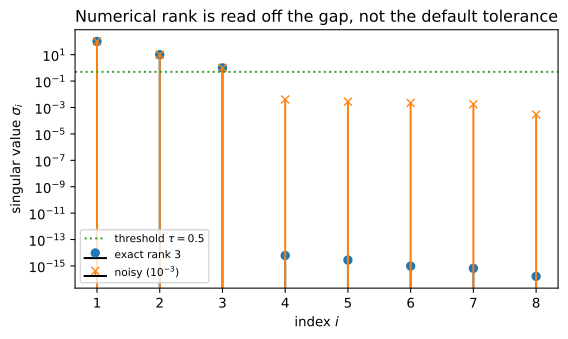
The exact spectrum decays as 10^2,10^1,10^0,0,0,\dots; the noisy spectrum replaces each trailing zero with a value near 10^{-3}. NumPy’s default tolerance, \sigma_1\,\varepsilon_{\text{mach}}\max(m,n)\approx10^{-13}, sits far below the noise floor, so the default declares the noisy matrix full rank (8) even though it is rank 3 in every meaningful sense. The correct reading is visual: the spectrum has a three-decade gap between \sigma_3=1 and \sigma_4\approx4\times10^{-3}, and any threshold placed inside that gap recovers the rank. The gap is what makes rank well-posed; without one, the number is a modeling choice rather than a fact of the data.
Full rank by shifting. A rank-deficient square matrix is a hair’s breadth from full rank: adding \lambda\mathbf{I} moves every eigenvalue by \lambda, so \mathbf{A}+\lambda\mathbf{I} is invertible whenever -\lambda is not an eigenvalue. This is the ridge shift behind regularization, the same operation that stabilizes least squares in Chapter 8. The tension is real: too large a \lambda makes \mathbf{A}+\lambda\mathbf{I}\approx\lambda\mathbf{I}, drowning the data; too small a \lambda leaves the matrix nearly singular. It is not a defect of the method but the unavoidable trade of a little bias for a lot of stability (the balance is struck in Chapters 8 and 10).
Demonstration: the CR decomposition. Starting from a known rank-r matrix and selecting its r pivot columns reproduces the factorization exactly. The code below verifies that the selected \mathbf{C} has independent columns and that \mathbf{C}\mathbf{R} reconstructs \mathbf{A} to machine precision.
import numpy as np
import scipy.linalg as la

rng = np.random.default_rng(1)
m, n, r = 6, 5, 3

C = rng.standard_normal((m, r))
R = rng.standard_normal((r, n))
A = C @ R                       # rank exactly r (generic)

# column-pivoted QR selects r independent columns of A
_, _, p = la.qr(A, pivoting=True, mode='economic')
piv = p[:r]                     # pivot columns
Csel = A[:, piv]
Rrec = np.linalg.lstsq(Csel, A, rcond=None)[0]

print('pivot columns      =', piv)
print('rank(Csel)         =', np.linalg.matrix_rank(Csel))
print('||A - Csel @ Rrec||=', np.linalg.norm(A - Csel @ Rrec))
pivot columns = [1 4 2]
rank(Csel) = 3
||A - Csel @ Rrec||= 3.0587302319905436e-15Column-pivoted QR chooses pivot columns that are maximally independent, and the least-squares solve then reads off the \mathbf{R} such that \mathbf{A}=\mathbf{C}_{\text{sel}}\mathbf{R}_{\text{rec}} to machine precision. The reconstruction error of about 10^{-15} confirms the exactness of the skeleton representation: a 6\times5 matrix carrying thirty entries is reproduced by three pivot columns and a 3\times5 coefficient matrix — thirty-three numbers in all, more than the original at this tiny size. The representation pays off only once the rank is small relative to both dimensions, r(m+n) \ll mn; this is the arithmetic behind low-rank compression.
The four fundamental subspaces
Every \mathbf{A}\in\mathbb{R}^{m\times n} induces four subspaces, two in each space:
| Subspace | Notation | Lives in | dimension |
|---|---|---|---|
| column space | \mathsf{C}(\mathbf{A}) | \mathbb{R}^m | r |
| null space | \mathsf{N}(\mathbf{A}) | \mathbb{R}^n | n-r |
| row space | \mathsf{C}(\mathbf{A}^{\mathsf T}) | \mathbb{R}^n | r |
| left null space | \mathsf{N}(\mathbf{A}^{\mathsf T}) | \mathbb{R}^m | m-r |
The dimensions in the right column come from rank-nullity applied to \mathbf{A} and to \mathbf{A}^{\mathsf T}, together with row rank equals column rank.
Theorem (fundamental theorem of linear algebra, I). The four subspaces decompose the input and output spaces orthogonally:
\mathbb{R}^n = \mathsf{C}(\mathbf{A}^{\mathsf T})\oplus\mathsf{N}(\mathbf{A}), \qquad \mathbb{R}^m = \mathsf{C}(\mathbf{A})\oplus\mathsf{N}(\mathbf{A}^{\mathsf T}),
with \mathsf{C}(\mathbf{A}^{\mathsf T})\perp\mathsf{N}(\mathbf{A}) and \mathsf{C}(\mathbf{A})\perp\mathsf{N}(\mathbf{A}^{\mathsf T}).
Proof. Orthogonality is the whole argument. A vector \mathbf{x} lies in \mathsf{N}(\mathbf{A}) exactly when \mathbf{A}\mathbf{x}=\mathbf{0}, that is, when \mathbf{x} is orthogonal to every row of \mathbf{A}; and the rows of \mathbf{A} span \mathsf{C}(\mathbf{A}^{\mathsf T}). Therefore
\mathsf{N}(\mathbf{A}) = \mathsf{C}(\mathbf{A}^{\mathsf T})^{\perp}.
Since a subspace and its orthogonal complement always satisfy V\oplus V^{\perp}=\mathbb{R}^n, the first decomposition follows. The second is the same sentence with \mathbf{A}^{\mathsf T} in place of \mathbf{A}. \square
Explicit bases via the SVD. Orthogonality is cheap; explicit bases need the SVD. With \mathbf{A}=\mathbf{U}\boldsymbol{\Sigma}\mathbf{V}^{\mathsf T} and r=\text{rank}(\mathbf{A}):
\mathsf{C}(\mathbf{A}^{\mathsf T}) = \operatorname{span}\{\mathbf{v}_1,\dots,\mathbf{v}_r\}, \qquad \mathsf{N}(\mathbf{A}) = \operatorname{span}\{\mathbf{v}_{r+1},\dots,\mathbf{v}_n\},
\mathsf{C}(\mathbf{A}) = \operatorname{span}\{\mathbf{u}_1,\dots,\mathbf{u}_r\}, \qquad \mathsf{N}(\mathbf{A}^{\mathsf T}) = \operatorname{span}\{\mathbf{u}_{r+1},\dots,\mathbf{u}_m\}.
Each line is verified directly: \mathbf{A}^{\mathsf T}\mathbf{u}_i=\sigma_i\mathbf{v}_i puts \mathbf{v}_1,\dots,\mathbf{v}_r in \mathsf{C}(\mathbf{A}^{\mathsf T}); \mathbf{A}\mathbf{v}_i=\mathbf{0} for i>r puts \mathbf{v}_{r+1},\dots,\mathbf{v}_n in \mathsf{N}(\mathbf{A}); and the counts (r and n-r) match the dimensions, so these spanning sets are bases. The same holds on the output side. This is the basis table of the four subspaces.
What a matrix does. Assembling the pieces: \mathbf{A} acts on \mathbb{R}^n=\mathsf{C}(\mathbf{A}^{\mathsf T})\oplus\mathsf{N}(\mathbf{A}) by
- carrying the row space \mathsf{C}(\mathbf{A}^{\mathsf T}) bijectively onto the column space \mathsf{C}(\mathbf{A}), stretching each direction \mathbf{v}_i by \sigma_i and rotating \mathbf{v}_i\mapsto\mathbf{u}_i;
- collapsing the null space \mathsf{N}(\mathbf{A}) entirely to \mathbf{0}.
This is the cleanest one-line summary of a linear map: rotate-and-stretch the information-carrying directions, annihilate the rest. The null space is the information \mathbf{A} destroys; the row space is the information it preserves.
import numpy as np
import matplotlib.pyplot as plt

rng = np.random.default_rng(2)
u = rng.standard_normal(2); u /= np.linalg.norm(u)
v = rng.standard_normal(2); v /= np.linalg.norm(v)
A = np.outer(u, v)                        # rank 1

x = np.array([0.8, 1.1])
x_row = (v @ x) * v                       # projection onto row space C(A^T)
x_nul = x - x_row                         # in N(A)

fig, ax = plt.subplots(figsize=(5.4, 5.4))
ax.axline((0, 0), v, color='C0', lw=1.5,
          label='row space $\\mathrm{C}(\\mathbf{A}^{\\mathrm{T}})$')
ax.axline((0, 0), np.array([-v[1], v[0]]), color='C1', lw=1.5,
          label='null space $\\mathrm{N}(\\mathbf{A})$')
ax.axline((0, 0), u, color='C2', lw=1.5, ls='--',
          label='column space $\\mathrm{C}(\\mathbf{A})$')

ax.quiver(0, 0, *x, angles='xy', scale_units='xy', scale=1, color='k', width=0.006)
ax.quiver(0, 0, *x_row, angles='xy', scale_units='xy', scale=1, color='C0', width=0.006)
ax.quiver(0, 0, *x_nul, angles='xy', scale_units='xy', scale=1, color='C1', width=0.006)
ax.quiver(0, 0, *(A @ x), angles='xy', scale_units='xy', scale=1, color='C2', width=0.006)

ax.annotate('$\\mathbf{x}$', x * 1.08)
ax.annotate('$\\mathbf{x}_{\\mathrm{row}}$', x_row * 1.05)
ax.annotate('$\\mathbf{x}_{\\mathrm{nul}}$', x_nul * 1.05)
ax.annotate('$\\mathbf{A}\\mathbf{x}$', (A @ x) * 1.1)

ax.set_xlim(-1.4, 1.4); ax.set_ylim(-1.4, 1.4)
ax.set_aspect('equal'); ax.grid(alpha=0.3)
ax.legend(loc='upper left', fontsize=8)
ax.set_title('$\\mathbf{A}\\mathbf{x} = \\mathbf{A}\\mathbf{x}_{\\mathrm{row}}$')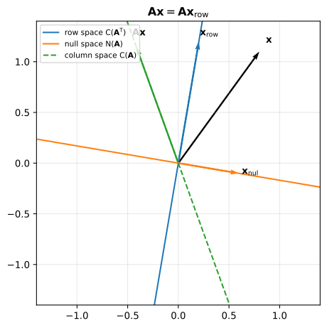
Solutions of \mathbf{A}\mathbf{x}=\mathbf{y}. The orthogonal decomposition makes the solution set of a linear system transparent. For \mathbf{y}\in\mathsf{C}(\mathbf{A}), the solutions are
\mathbf{x} = \mathbf{h} + \sum_{k=1}^{n-r} c_k \mathbf{v}_{r+k},
where \mathbf{h} is any single (particular) solution and the c_k are n-r free parameters ranging over the null space. In the row-reduction picture the coordinates c_k are the free variables, and each basis vector \mathbf{v}_{r+k} solves the homogeneous system \mathbf{A}\mathbf{x}=\mathbf{0} while \mathbf{h} is the particular solution of \mathbf{A}\mathbf{x}=\mathbf{y}. The particular solution of smallest norm is the one with zero null-space component, \mathbf{h}\in\mathsf{C}(\mathbf{A}^{\mathsf T}): the minimum-norm solution \mathbf{x}^{\dagger}=\mathbf{V}_r\boldsymbol{\Sigma}_r^{-1}\mathbf{U}_r^{\mathsf T}\mathbf{y}, the pseudoinverse of Chapter 6.
import numpy as np

rng = np.random.default_rng(3)
m, n, r = 4, 5, 2

U, _ = np.linalg.qr(rng.standard_normal((m, r)))
V, _ = np.linalg.qr(rng.standard_normal((n, r)))
sig = np.array([3.0, 1.0])
A = (U * sig) @ V.T                       # rank 2, shape 4x5

y = A @ rng.standard_normal(n)            # a right-hand side in C(A)

u, s, vh = np.linalg.svd(A, full_matrices=False)
x_dag = (vh[:r].T / s[:r]) @ (u[:, :r].T @ y)  # minimum-norm solution (preview of Ch.6)

null_basis = vh[r:].T                     # (n, n-r) columns span N(A)
c = np.array([[0.0, 0.0], [1.0, -0.5], [-2.0, 0.7]])
solns = x_dag[:, None] + null_basis @ c.T # (n, 3) shifted solutions

residuals = A @ solns - y[:, None]
print('||A @ x_dag - y||        =', np.linalg.norm(A @ x_dag - y))
print('max ||A @ x_k - y|| over 3 =', np.max(np.linalg.norm(residuals, axis=0)))
print('norms (min-norm, shifted) =',
      np.round([np.linalg.norm(x_dag), *np.linalg.norm(solns, axis=0)], 4))
||A @ x_dag - y|| = 4.577566798522237e-16
max ||A @ x_k - y|| over 3 = 6.377745716588144e-16
norms (min-norm, shifted) = [1.5079 1.5079 1.8772 2.6007]Every solution is \mathbf{x}^{\dagger} plus a point of the null space, so all three shifted vectors reproduce \mathbf{y} exactly (residual about 10^{-15}); the two nonzero shifts have norms strictly exceeding \|\mathbf{x}^{\dagger}\|, while the first shift lands exactly on \mathbf{x}^{\dagger} because its coefficient vector is zero — confirming that the SVD’s particular solution is the minimum-norm one. The null space is the ambiguity in the system, the information \mathbf{y} cannot pin down; the row space is the information it does.
Summary
- Rank is the dimension of the image; it is well-defined because the exchange lemma forces all bases to share a cardinality.
- Rank-nullity, \dim\mathsf{N}(\mathbf{A})+\text{rank}(\mathbf{A})=n, is the accounting identity of a linear map.
- Row rank equals column rank, provable abstractly through \mathsf{N}(\mathbf{A}^{\mathsf T}\mathbf{A})=\mathsf{N}(\mathbf{A}) and read off instantly from the SVD.
- Numerically, rank is a count at a tolerance: the singular-value spectrum and its gaps decide how well-posed the question is.
- The four fundamental subspaces decompose \mathbb{R}^n and \mathbb{R}^m orthogonally; the SVD supplies explicit bases. A matrix rotates-and-stretches its row space onto its column space and annihilates its null space.
- The solution set of \mathbf{A}\mathbf{x}=\mathbf{y} is a particular solution plus the null space; the minimum-norm member is the pseudoinverse of Chapter 6.
Problems
Each problem uses the notation of this chapter: \mathsf{C}(\cdot) for column and row spaces, \mathsf{N}(\cdot) for null spaces, and \text{rank}(\cdot) for the common dimension. Problems 1–2 are theory, 3–4 are short numerical checks, and Problem 5 is a numerical experiment.
[P4.1] Rank of a product
Let \mathbf{A}\in\mathbb{R}^{m\times n} and \mathbf{B}\in\mathbb{R}^{n\times p}.
Prove \text{rank}(\mathbf{A}\mathbf{B})\le\text{rank}(\mathbf{A}) by showing that every column of \mathbf{A}\mathbf{B} is a linear combination of the columns of \mathbf{A}, hence \mathsf{C}(\mathbf{A}\mathbf{B})\subseteq\mathsf{C}(\mathbf{A}).
Prove \text{rank}(\mathbf{A}\mathbf{B})\le\text{rank}(\mathbf{B}) by applying part (a) to the transposes and using row rank equals column rank.
Suppose \mathbf{A} has full column rank, \text{rank}(\mathbf{A})=n. Prove \text{rank}(\mathbf{A}\mathbf{B})=\text{rank}(\mathbf{B}). Hint: show \mathsf{N}(\mathbf{A}\mathbf{B})=\mathsf{N}(\mathbf{B}) and apply rank-nullity.
[P4.2] The subspaces of \mathbf{A}^{\mathsf T}\mathbf{A}
Let \mathbf{A}\in\mathbb{R}^{m\times n}.
Prove \mathsf{N}(\mathbf{A}\mathbf{A}^{\mathsf T})=\mathsf{N}(\mathbf{A}^{\mathsf T}) by the norm argument used in the chapter for \mathbf{A}^{\mathsf T}\mathbf{A}: if \mathbf{A}\mathbf{A}^{\mathsf T}\mathbf{x}=\mathbf{0}, then \lVert\mathbf{A}^{\mathsf T}\mathbf{x}\rVert^2=\mathbf{x}^{\mathsf T}\mathbf{A}\mathbf{A}^{\mathsf T}\mathbf{x}=0.
Prove \mathsf{C}(\mathbf{A}^{\mathsf T}\mathbf{A})=\mathsf{C}(\mathbf{A}^{\mathsf T}) and \mathsf{C}(\mathbf{A}\mathbf{A}^{\mathsf T})=\mathsf{C}(\mathbf{A}). Hint: take orthogonal complements in part (a) and in the chapter’s identity \mathsf{N}(\mathbf{A}^{\mathsf T}\mathbf{A})=\mathsf{N}(\mathbf{A}), then apply the fundamental theorem of linear algebra.
Conclude \text{rank}(\mathbf{A}^{\mathsf T}\mathbf{A})=\text{rank}(\mathbf{A})=\text{rank}(\mathbf{A}\mathbf{A}^{\mathsf T}).
[P4.3] Numerical rank from the spectrum
Construct an 8\times8 matrix \mathbf{A} of exact rank 3 with singular values 10^2,10^1,10^0, then add 10^{-3} additive noise. Compare three rank estimates: the exact rank, the default-tolerance rank of the noisy matrix, and the rank at a threshold placed inside the spectral gap. The starter code below prints all three alongside the noisy spectrum.
import numpy as np

rng = np.random.default_rng(0)
m = n = 8
sigma = np.array([1e2, 1e1, 1e0])

U, _ = np.linalg.qr(rng.standard_normal((m, 3)))
V, _ = np.linalg.qr(rng.standard_normal((n, 3)))
A = (U * sigma) @ V.T
An = A + 1e-3 * rng.standard_normal((m, n))

s = np.linalg.svd(An, compute_uv=False)

rank_exact = np.linalg.matrix_rank(A)
rank_default = np.linalg.matrix_rank(An)
rank_gap = np.linalg.matrix_rank(An, tol=0.5)

print('rank(exact)              =', rank_exact)
print('rank(noisy, default tol) =', rank_default)
print('rank(noisy, tol=0.5)     =', rank_gap)
print('sigma(noisy)             =', np.round(s, 4))
rank(exact) = 3
rank(noisy, default tol) = 8
rank(noisy, tol=0.5) = 3
sigma(noisy) = [9.99996e+01 9.99940e+00 1.00040e+00 4.00000e-03 2.80000e-03 2.20000e-03
1.80000e-03 3.00000e-04]The exact spectrum is 10^2,10^1,10^0,0,\dots; the noisy spectrum replaces the trailing zeros with values near 10^{-3}. The default tolerance sits below the noise floor and declares the noisy matrix full rank, while a threshold inside the three-decade gap recovers the true rank 3.
[P4.4] The CR decomposition
Build a rank-3 matrix \mathbf{A}=\mathbf{C}\mathbf{R} with \mathbf{C}\in\mathbb{R}^{6\times3} and \mathbf{R}\in\mathbb{R}^{3\times5}, then recover the skeleton: select the r pivot columns of \mathbf{A} by column-pivoted QR and solve for the coefficient matrix. The starter code below prints the pivot columns, the rank of the selected column matrix, and the reconstruction error.
import numpy as np
import scipy.linalg as la

rng = np.random.default_rng(1)
m, n, r = 6, 5, 3

C = rng.standard_normal((m, r))
R = rng.standard_normal((r, n))
A = C @ R

_, _, p = la.qr(A, pivoting=True, mode='economic')
piv = p[:r]
Csel = A[:, piv]
Rrec = np.linalg.lstsq(Csel, A, rcond=None)[0]

print('pivot columns      =', piv)
print('rank(Csel)         =', np.linalg.matrix_rank(Csel))
print('||A - Csel @ Rrec||=', np.linalg.norm(A - Csel @ Rrec))
pivot columns = [1 4 2]
rank(Csel) = 3
||A - Csel @ Rrec||= 3.0587302319905436e-15The selected columns are maximally independent, so \text{rank}(\mathbf{C}_{\text{sel}})=3, and the least-squares solve recovers \mathbf{R} to machine precision: the reconstruction error sits near 10^{-15}, confirming the exactness of the skeleton representation.
[P4.5] The gap decides the rank
Challenge. The chapter’s figure examines a single noise level. This experiment sweeps the noise floor and locates where the rank stops being well-posed.
For each \varepsilon\in\{10^{-1},10^{-3},10^{-5}\}, build the rank-3 matrix of Problem 3, add \varepsilon times standard-normal noise, and record \sigma_3 and \sigma_4 of the noisy matrix.
For each \varepsilon, place a threshold at the geometric midpoint \tau=\sqrt{\sigma_3\sigma_4} of the gap and report the numerical rank at that threshold, alongside the default-tolerance rank.
Repeat with \varepsilon=1. Report \sigma_3,\sigma_4 and both ranks. The gap threshold still returns rank 3, but the recovered rank is now spurious: explain in one sentence why, given that \sigma_4 exceeds the smallest genuine singular value \sigma_3(\mathbf{A})=1. The starter code below runs the whole sweep.
import numpy as np

rng = np.random.default_rng(0)
m = n = 8
sigma = np.array([1e2, 1e1, 1e0])

U, _ = np.linalg.qr(rng.standard_normal((m, 3)))
V, _ = np.linalg.qr(rng.standard_normal((n, 3)))
A = (U * sigma) @ V.T

for eps in [1e-1, 1e-3, 1e-5, 1.0]:
    An = A + eps * rng.standard_normal((m, n))
    s = np.linalg.svd(An, compute_uv=False)
    s3, s4 = s[2], s[3]
    tau = np.sqrt(s3 * s4)
    rank_gap = np.linalg.matrix_rank(An, tol=tau)
    rank_default = np.linalg.matrix_rank(An)
    print(f'eps={eps:6.1e}  sigma3={s3:9.4f}  sigma4={s4:9.4f}  '
          f'rank(tau)={rank_gap}  rank(default)={rank_default}')
eps=1.0e-01 sigma3= 1.0749 sigma4= 0.4020 rank(tau)=3 rank(default)=8
eps=1.0e-03 sigma3= 1.0000 sigma4= 0.0032 rank(tau)=3 rank(default)=8
eps=1.0e-05 sigma3= 1.0000 sigma4= 0.0000 rank(tau)=3 rank(default)=8
eps=1.0e+00 sigma3= 4.8870 sigma4= 3.3216 rank(tau)=3 rank(default)=8For \varepsilon\le10^{-1} the noise floor \sigma_4 sits below the smallest genuine singular value \sigma_3(\mathbf{A})=1, so the gap threshold recovers the true rank 3 while the default tolerance reports 8. At \varepsilon=1 the noise floor (\sigma_4\approx3.3) exceeds \sigma_3(\mathbf{A})=1: the third singular value of the noisy matrix is a noise direction, so the rank 3 recovered by the gap threshold is spurious and the matrix is genuinely full rank.