from watchtower.core import set_format
set_format("svg")Least squares
Given a design matrix \mathbf{X} \in \mathbb{R}^{n\times d} and observations \mathbf{y}\in\mathbb{R}^n, the least-squares problem asks for the coefficient vector \mathbf{w}\in\mathbb{R}^d that makes \mathbf{X}\mathbf{w} as close as possible to \mathbf{y}:
\boxed{\ \hat{\mathbf{w}} = \operatorname*{arg\,min}_{\mathbf{w}\in\mathbb{R}^d}\ \lVert \mathbf{X}\mathbf{w} - \mathbf{y} \rVert^2\ }
The model \mathbf{X}\mathbf{w} = \mathbf{w}_1\mathbf{x}_1 + \cdots + \mathbf{w}_d\mathbf{x}_d is a linear combination of the columns of \mathbf{X}, so geometrically this is the same question that Chapter 7 already answered: find the closest point of \mathsf{C}(\mathbf{X}) to \mathbf{y}, and express it in the column basis. What makes this chapter its own subject is the data interpretation. Each row of \mathbf{X} is one observation of d input features, each entry of \mathbf{y} is the corresponding measured output, and \mathbf{w} are the unknown parameters of a linear model fit to those n samples. The same mathematics then connects directly to optimization. The objective is a convex quadratic, the natural arena for gradient descent, and the geometry of its minima is governed entirely by the rank of \mathbf{X}.
The objective and its gradient
Write the loss as a sum over the n samples:
J(\mathbf{w}) = \lVert \mathbf{X}\mathbf{w} - \mathbf{y}\rVert^2 = \sum_{i=1}^{n}\Big(\mathbf{z}_i^{\mathsf T}\mathbf{w} - y_i\Big)^2 .
Here \mathbf{z}_i^{\mathsf T} denotes the i-th row of \mathbf{X}, the d features measured on sample i. The columns of \mathbf{X} are denoted \mathbf{x}_1,\dots,\mathbf{x}_d: column \mathbf{x}_j stacks the j-th feature across all n samples, so z_{ij} = x_{ji} is the entry of \mathbf{X} in row i, column j. Expanding and collecting terms gives a quadratic form in \mathbf{w}:
J(\mathbf{w}) = \mathbf{w}^{\mathsf T}\mathbf{X}^{\mathsf T}\mathbf{X}\mathbf{w} - 2\mathbf{y}^{\mathsf T}\mathbf{X}\mathbf{w} + \mathbf{y}^{\mathsf T}\mathbf{y},
whose gradient and Hessian are
\nabla J(\mathbf{w}) = 2\mathbf{X}^{\mathsf T}\left(\mathbf{X}\mathbf{w} - \mathbf{y}\right), \qquad \nabla^2 J(\mathbf{w}) = 2\mathbf{X}^{\mathsf T}\mathbf{X}.
The Hessian is a Gram matrix, hence positive semidefinite by Chapter 3, so J is convex. Setting the gradient to zero yields the normal equations,
\boxed{\ \mathbf{X}^{\mathsf T}\mathbf{X}\,\mathbf{w} = \mathbf{X}^{\mathsf T}\mathbf{y}.\ }
Any stationary point of a convex function is a global minimizer, so solving the normal equations is solving the least-squares problem. When the columns of \mathbf{X} are linearly independent, \mathbf{X}^{\mathsf T}\mathbf{X} is invertible (its null space equals \mathsf{N}(\mathbf{X}) by the argument in Chapter 4), and the solution is unique:
\hat{\mathbf{w}} = \left(\mathbf{X}^{\mathsf T}\mathbf{X}\right)^{-1}\mathbf{X}^{\mathsf T}\mathbf{y}.
The product \mathbf{X}\hat{\mathbf{w}} is then exactly the orthogonal projection of \mathbf{y} onto \mathsf{C}(\mathbf{X}) from Chapter 7, confirming the geometric reading.
The SVD solution and non-uniqueness
The normal equations are elegant but fragile: forming \mathbf{X}^{\mathsf T}\mathbf{X} squares the condition number, \kappa(\mathbf{X}^{\mathsf T}\mathbf{X}) = \kappa(\mathbf{X})^2, so solving them can lose accuracy. The SVD gives a solution that sidesteps this. Writing \mathbf{X} = \mathbf{U}\boldsymbol{\Sigma}\mathbf{V}^{\mathsf T} and rotating to the singular-vector coordinates \mathbf{z} = \mathbf{V}^{\mathsf T}\mathbf{w}, \mathbf{c} = \mathbf{U}^{\mathsf T}\mathbf{y},
\lVert \mathbf{X}\mathbf{w} - \mathbf{y}\rVert^2 = \lVert \boldsymbol{\Sigma}\mathbf{z} - \mathbf{c}\rVert^2 = \sum_{i=1}^{r}\left(\sigma_i z_i - c_i\right)^2 + \sum_{i=r+1}^{n} c_i^2 .
The second sum is the irreducible distance from \mathbf{y} to \mathsf{C}(\mathbf{X}); it does not depend on \mathbf{w}. The first sum vanishes by taking z_i = c_i/\sigma_i for i \le r, while z_{r+1},\dots,z_d are completely unconstrained. In the original coordinates this reads
\boxed{\ \hat{\mathbf{w}} = \mathbf{X}^{+}\mathbf{y} + \sum_{j=r+1}^{d}\alpha_j\,\mathbf{v}_j, \qquad \alpha_j \in \mathbb{R}.\ }
The pseudoinverse term \mathbf{X}^{+}\mathbf{y} is the minimum-norm solution (it has no component along the null space \mathsf{N}(\mathbf{X}) = \operatorname{span}\{\mathbf{v}_{r+1},\dots,\mathbf{v}_d\}), and the homogeneous terms trace out the whole affine space of minimizers. Uniqueness is therefore a rank statement: the minimizer is unique exactly when r = d, i.e. the columns of \mathbf{X} are independent; otherwise the optimal weights form a (d-r)-dimensional affine subspace.
Gradient descent
Because the loss is a convex quadratic, it is also the natural first example of iterative optimization. The gradient-descent update moves \mathbf{w} against the gradient with a fixed step size \eta:
\mathbf{w}^{(t+1)} = \mathbf{w}^{(t)} - \eta\,\nabla J\left(\mathbf{w}^{(t)}\right), \qquad \nabla J(\mathbf{w}) = \frac{2}{n}\sum_{i=1}^{n}\left(\mathbf{z}_i^{\mathsf T}\mathbf{w} - y_i\right)\mathbf{z}_i .
This is exactly a linear model trained with mean-squared-error loss, the simplest possible neural network, with identity activation. The update is cheap to vectorize: dotting each column of \mathbf{X} with the residual \mathbf{X}\mathbf{w} - \mathbf{y} produces the full gradient at once. The next cell fits the line y = -1 + 3x under Gaussian noise and traces the descent of the iterates.
import numpy as np
import matplotlib.pyplot as plt

rng = np.random.default_rng(0)

def loss(w, X, y):
    """Mean-squared-error loss."""
    return ((X @ w - y) ** 2).mean()

def grad(w, X, y):
    """Full-batch gradient, vectorized: 2/n * X^T (X w - y)."""
    return 2 / X.shape[0] * X.T @ (X @ w - y)

# Signal: y = -1 + 3 x + noise
n = 1000
X = np.column_stack([np.ones(n), rng.uniform(-1, 1, size=n)])
w_true = np.array([-1.0, 3.0])
y = X @ w_true + 0.01 * rng.standard_normal(n)

# Gradient descent from a deliberately bad start
w = np.array([-4.0, -4.0])
eta, epochs = 0.6, 20
w_hist, loss_hist = [w.copy()], [loss(w, X, y)]
for _ in range(epochs):
    w = w - eta * grad(w, X, y)
    w_hist.append(w.copy())
    loss_hist.append(loss(w, X, y))
w_hist = np.array(w_hist)

# Loss landscape over a grid
g = np.linspace(-5, 5, 200)
W0, W1 = np.meshgrid(g, g)
Z = np.array([[loss(np.array([a, b]), X, y) for a in g] for b in g])

fig, ax = plt.subplots(1, 2, figsize=(10, 4))
ax[0].plot(loss_hist, 'o--', color='firebrick', ms=4)
ax[0].set_xlabel('iteration')
ax[0].set_ylabel('loss')
ax[1].contourf(W0, W1, Z, levels=30, cmap='Reds')
ax[1].plot(w_hist[:, 0], w_hist[:, 1], 'k-o', ms=3, lw=0.8)
ax[1].plot(*w_true, 'k*', ms=14)
ax[1].set_xlabel('$w_0$')
ax[1].set_ylabel('$w_1$')
fig.tight_layout()
plt.show()

w_pinv = np.linalg.pinv(X) @ y
print('MSE(w_true)       =', f'{loss(w_true, X, y):.3e}')
print('MSE(w after GD)   =', f'{loss(w_hist[-1], X, y):.3e}')
print('MSE(pinv)         =', f'{loss(w_pinv, X, y):.3e}')
print('w_true  =', w_true)
print('w_pinv  =', np.round(w_pinv, 4))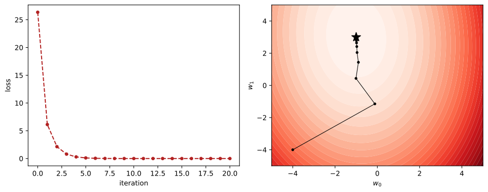
MSE(w_true)       = 1.052e-04
MSE(w after GD)   = 1.052e-04
MSE(pinv)         = 1.052e-04
w_true  = [-1.  3.]
w_pinv  = [-1.0001  2.9999]
Gradient descent on a convex quadratic.
The annotations: <1> prepends a column of ones so the first coefficient is an intercept (the bias term). Three quantities deserve comment.
First, gradient descent reaches essentially the same loss as the exact pseudoinverse solution even though it never forms \mathbf{X}^{+}; in the right panel, the star marks \mathbf{w}_{\text{true}} and the black path shows the iterates converging to it. Second, the best achievable loss is not zero. The residual \mathbf{y} - \mathbf{X}\hat{\mathbf{w}} at the optimum is the noise with its component along the d-dimensional column space removed, so only the n - d complementary directions contribute: its expected squared norm is (n-d)\sigma^2. With n = 1000 samples, d = 2 parameters and \sigma = 0.01 the expected loss is \mathbb{E}[J(\hat{\mathbf{w}})] = \tfrac{n-d}{n}\sigma^2 = 9.98\times 10^{-5}, and the printed values are a single draw fluctuating around that mean.
Third, because the columns of \mathbf{X} are independent, the minimum is unique and the basin is a single well; the next section shows what changes when they are not.
Loss surfaces and the rank of \mathbf{X}
When the columns of \mathbf{X} are dependent, \mathbf{X}^{\mathsf T}\mathbf{X} is singular, the Hessian has a zero eigenvalue, and the minimizer is no longer unique: the loss is flat along \mathsf{N}(\mathbf{X}), so the optimum is a valley rather than a point. The contrast is easiest to see in d = 2, where the optimal set is a line. The figure below compares a full-rank design (\mathbf{X} = [\mathbf{1},\ \mathbf{x}]) against a rank-one design (\mathbf{X} = [2\mathbf{x},\ \mathbf{x}], so r = 1 < d = 2).
def plot_surface(X, y, ax):
    g = np.linspace(-6, 6, 250)
    W0, W1 = np.meshgrid(g, g)
    Z = np.array([[loss(np.array([a, b]), X, y) for a in g] for b in g])
    ax.contourf(W0, W1, Z, levels=30, cmap='Reds')
    # draw the optimal set  w = pinv(X)y + alpha * v2
    u, s, vt = np.linalg.svd(X, full_matrices=False)
    r = np.count_nonzero(s > 1e-8)
    w0 = np.linalg.pinv(X) @ y
    alphas = np.linspace(-6, 6, 100)
    pts = [w0]                                        # <2> the min-norm solution
    for j in range(r, 2):                             # <3> null-space directions v_{r+1..d}
        pts.extend(w0 + a * vt[j] for a in alphas)
    pts = np.array(pts)
    ax.plot(pts[:, 0], pts[:, 1], 'k.', ms=0.8)
    ax.set_xlabel('$w_0$'); ax.set_ylabel('$w_1$')

n = 1000
x = rng.uniform(-1, 1, size=n)
fig, ax = plt.subplots(1, 2, figsize=(10, 4))

# Independent columns: r = d = 2 -> unique minimum
X_ind = np.column_stack([np.ones(n), x])
y_ind = X_ind @ w_true + 0.01 * rng.standard_normal(n)
plot_surface(X_ind, y_ind, ax[0])
ax[0].set_title('independent columns: unique minimum')

# Dependent columns: r = 1 < d = 2 -> a line of minima
X_dep = np.column_stack([2 * x, x])
y_dep = X_dep @ w_true + 0.01 * rng.standard_normal(n)
plot_surface(X_dep, y_dep, ax[1])
ax[1].set_title('dependent columns: a valley of minima')

fig.tight_layout()
plt.show()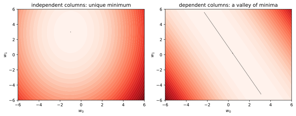
Unique versus non-unique minima. The annotations: <2> seeds the plot with the min-norm solution \mathbf{X}^{+}\mathbf{y}, and <3> sweeps the null-space directions \mathbf{v}_{r+1},\dots,\mathbf{v}_d from the SVD to generate the rest of the optimal set. The left panel has independent columns, so r = d and the black dots collapse to a single minimum. The right panel has dependent columns (\mathbf{x}_1 = 2\mathbf{x}_2), so the loss is flat along \mathbf{v}_2 and the minimizers form a one-dimensional ridge: every point on that line achieves the same loss. This is exactly the affine set \hat{\mathbf{w}} = \mathbf{X}^{+}\mathbf{y} + \alpha\mathbf{v}_2 predicted by the SVD solution. Rank deficiency is what makes the normal equations \mathbf{X}^{\mathsf T}\mathbf{X}\mathbf{w} = \mathbf{X}^{\mathsf T}\mathbf{y} singular here, and every point of the ridge is one of their infinitely many solutions.
Conditioning and convergence
Two numerical lessons follow from the fact that the Hessian is \mathbf{X}^{\mathsf T}\mathbf{X}. Its condition number is \kappa(\mathbf{X}^{\mathsf T}\mathbf{X}) = \kappa(\mathbf{X})^2 = (\sigma_1/\sigma_d)^2, so a design matrix that is merely moderately ill-conditioned produces a very ill-conditioned normal-equation system: squaring \kappa doubles its exponent. This is why forming and solving \mathbf{X}^{\mathsf T}\mathbf{X} is discouraged in favor of QR- or SVD-based solvers, which work with \mathbf{X} directly. The same quantity governs gradient descent: on a quadratic with condition number \kappa, the best achievable linear convergence rate is (\kappa - 1)/(\kappa + 1), so a large \kappa(\mathbf{X}) makes the iterates crawl. Scaling or regularizing the features — replacing \mathbf{X}^{\mathsf T}\mathbf{X} by \mathbf{X}^{\mathsf T}\mathbf{X} + \lambda\mathbf{I} — both improve the condition number, at the cost of a small bias. Regularization is the subject of Chapter 10, where the shifted spectrum of \mathbf{X}^{\mathsf T}\mathbf{X} + \lambda\mathbf{I} is examined directly.
# Condition number governs both solver stability and GD speed.
kappa_gram = lambda X: np.linalg.cond(X) ** 2

for name, X in [('well-scaled', X_ind), ('rank-deficient', X_dep)]:
    g = np.linalg.cond(X)
    print(f'{name:>15}: kappa(X) = {g:10.2e},  kappa(X^T X) = {kappa_gram(X):10.2e}')

# A nearly-collinear design: x2 = x1 + tiny noise
x1 = rng.uniform(-1, 1, size=n)
X_bad = np.column_stack([x1, x1 + 1e-8 * rng.standard_normal(n)])
y_bad = X_bad @ np.array([2.0, -1.0]) + 0.01 * rng.standard_normal(n)
print(f'{"nearly-collinear":>15}: kappa(X) = {np.linalg.cond(X_bad):10.2e},'
      f'  kappa(X^T X) = {kappa_gram(X_bad):10.2e}')
well-scaled: kappa(X) = 1.75e+00, kappa(X^T X) = 3.06e+00
rank-deficient: kappa(X) = 1.02e+16, kappa(X^T X) = 1.04e+32
nearly-collinear: kappa(X) = 1.15e+08, kappa(X^T X) = 1.32e+16The nearly-collinear design has two columns that agree to within 10^{-8}, so the direction distinguishing them is 10^{-8} times as prominent as the common direction, and \kappa(\mathbf{X}) \approx 10^{8}. Squaring for the normal equations yields \kappa(\mathbf{X}^{\mathsf T}\mathbf{X}) \approx 10^{16}, at the very edge of double-precision resolution. Solving the normal equations for such a matrix would be hopeless, yet the SVD-based pseudoinverse remains accurate because it works directly with \mathbf{X} and never squares the condition number. This single example is the practical justification for preferring \mathbf{X}^{+} over (\mathbf{X}^{\mathsf T}\mathbf{X})^{-1}\mathbf{X}^{\mathsf T}.
Summary
The least-squares solution of \lVert\mathbf{X}\mathbf{w}-\mathbf{y}\rVert^2 is the orthogonal projection of \mathbf{y} onto \mathsf{C}(\mathbf{X}), and is computed either by the normal equations \mathbf{X}^{\mathsf T}\mathbf{X}\mathbf{w} = \mathbf{X}^{\mathsf T}\mathbf{y} or, more stably, by the pseudoinverse \hat{\mathbf{w}} = \mathbf{X}^{+}\mathbf{y}. The objective is a convex quadratic whose Hessian is the Gram matrix \mathbf{X}^{\mathsf T}\mathbf{X}; uniqueness of the minimizer is equivalent to \mathbf{X} having independent columns, and otherwise the minima form a (d-r)-dimensional affine subspace of the parameter space. Gradient descent finds the minimum iteratively without forming any inverse, converging at a rate set by \kappa(\mathbf{X})^2, the same quantity that makes the normal equations numerically fragile. These three views — geometry (projection), algebra (normal equations and the SVD), and optimization (gradient descent on a convex quadratic) — are one theorem seen from three directions.
Problems
The problems below exercise the least-squares theory, the conditioning of the normal equations, and gradient descent. Problems 1-2 are derivations, Problems 3-4 are numerical, and Problem 5 is a challenge experiment.
[P8.1] The expected loss at the optimum
Let \mathbf X\in\mathbb R^{n\times d} have full column rank with n>d, and let \mathbf y=\mathbf X\mathbf w_{\text{true}}+\boldsymbol\varepsilon, where the entries of \boldsymbol\varepsilon are independent with \mathbb E[\varepsilon_i]=0 and \operatorname{Var}(\varepsilon_i)=\sigma^2. Let \hat{\mathbf w} be the least-squares solution and P=\mathbf X(\mathbf X^{\mathsf T}\mathbf X)^{-1}\mathbf X^{\mathsf T} the projector onto \mathsf C(\mathbf X).
Show that the residual \mathbf e=\mathbf y-\mathbf X\hat{\mathbf w} satisfies \mathbf X^{\mathsf T}\mathbf e=\mathbf 0, so \mathbf e\perp\mathsf C(\mathbf X).
Show that \mathbf e=(\mathbf I-P)\boldsymbol\varepsilon. Hint: \mathbf X\hat{\mathbf w}=P\mathbf y and P\mathbf X=\mathbf X.
Using \operatorname{tr}P=d and \mathbb E[\boldsymbol\varepsilon\boldsymbol\varepsilon^{\mathsf T}]=\sigma^2\mathbf I, show that
\mathbb E[\lVert\mathbf e\rVert^2]=(n-d)\sigma^2,
and hence that the mean-squared-error loss J(\mathbf w)=\frac1n\lVert\mathbf X\mathbf w-\mathbf y\rVert^2 satisfies \mathbb E[J(\hat{\mathbf w})]=\frac{n-d}{n}\sigma^2, the value the chapter’s gradient-descent demo fluctuates around.
[P8.2] The geometry of non-uniqueness
Let \mathbf X\in\mathbb R^{n\times d} have rank r<d.
Show that if \hat{\mathbf w}_1,\hat{\mathbf w}_2 both minimize \lVert\mathbf X\mathbf w-\mathbf y\rVert^2, then \hat{\mathbf w}_1-\hat{\mathbf w}_2\in\mathsf N(\mathbf X). Hint: both satisfy the normal equations, and \mathsf N(\mathbf X^{\mathsf T}\mathbf X)=\mathsf N(\mathbf X).
Using the SVD \mathbf X=\mathbf U\boldsymbol\Sigma\mathbf V^{\mathsf T}, write an arbitrary minimizer as \mathbf w=\mathbf X^{+}\mathbf y+\sum_{j=r+1}^{d}\alpha_j\mathbf v_j and show that
\lVert\mathbf w\rVert^2=\lVert\mathbf X^{+}\mathbf y\rVert^2+\sum_{j=r+1}^{d}\alpha_j^2.
Conclude that the minimum-norm minimizer is \mathbf X^{+}\mathbf y.
- Conclude that the set of minimizers is the affine subspace \mathbf X^{+}\mathbf y+\mathsf N(\mathbf X) of dimension d-r.
[P8.3] Normal equations vs pseudoinverse
The chapter’s nearly-collinear design has \mathbf x_2=\mathbf x_1+10^{-8}\cdot noise, giving \kappa(\mathbf X)\approx 10^8 and \kappa(\mathbf X^{\mathsf T}\mathbf X)\approx 10^{16}. This problem compares the normal equations against the pseudoinverse on that design.
Build the design and solve for \mathbf w three ways: the normal equations
np.linalg.solve(X.T @ X, X.T @ y), the pseudoinversenp.linalg.pinv(X) @ y, andnp.linalg.lstsq. Report \kappa(\mathbf X), \kappa(\mathbf X^{\mathsf T}\mathbf X), and their ratio.Compare the solutions: the relative difference \lVert\mathbf w_{\text{ne}}-\mathbf w_{\text{pinv}}\rVert/\lVert\mathbf w_{\text{pinv}}\rVert should be large, because the weights are not identifiable when the columns are nearly collinear, while
lstsqshould agree with the pseudoinverse to machine precision.Compare the losses J(\mathbf w)=\frac1n\lVert\mathbf X\mathbf w-\mathbf y\rVert^2 at the three solutions: all sit near the minimum, showing that a wildly wrong \mathbf w can still fit well.
The starter code builds the data; fill in the measurements.
import numpy as np

rng = np.random.default_rng(3)
n = 1000
x1 = rng.uniform(-1, 1, size=n)
X = np.column_stack([x1, x1 + 1e-8 * rng.standard_normal(n)])
w_true = np.array([2.0, -1.0])
y = X @ w_true + 0.01 * rng.standard_normal(n)

# (a) kappa(X), kappa(X^T X), and their ratio
# (b) w_ne, w_pinv, w_lstsq; relative differences
# (c) losses J(w) = ((X @ w - y) ** 2).mean() for each solution
[P8.4] Gradient descent: rate vs condition number
The chapter states that on a quadratic with Hessian condition number \kappa, gradient descent with the optimal step converges at the linear rate (\kappa-1)/(\kappa+1). This problem verifies that rate numerically on a design with prescribed singular values.
Build \mathbf X=\mathbf U\operatorname{diag}(\sigma_1,\dots,\sigma_d)\mathbf V^{\mathsf T} with n=300, d=6, and singular values log-spaced from 1 to 1/\kappa(\mathbf X) with \kappa(\mathbf X)=10. The Hessian of J(\mathbf w)=\frac1n\lVert\mathbf X\mathbf w-\mathbf y\rVert^2 is \frac2n\mathbf X^{\mathsf T}\mathbf X, so \kappa(\nabla^2 J)=\kappa(\mathbf X)^2=100 and the predicted rate is 99/101\approx 0.9802.
Run gradient descent from \mathbf w^{(0)}=\mathbf 0 with the optimal step \eta=2/(\lambda_{\max}+\lambda_{\min}), where \lambda_{\max},\lambda_{\min} are the extreme eigenvalues of \frac2n\mathbf X^{\mathsf T}\mathbf X. Record \lVert\mathbf w^{(t)}-\hat{\mathbf w}\rVert against the exact solution \hat{\mathbf w}=\mathbf X^{+}\mathbf y, and estimate the empirical contraction factor \hat\rho=(\lVert\mathbf w^{(T)}-\hat{\mathbf w}\rVert/\lVert\mathbf w^{(0)}-\hat{\mathbf w}\rVert)^{1/T}.
Compare \hat\rho with (\kappa-1)/(\kappa+1), and confirm that the step \eta=2.5/\lambda_{\max}, past the stability limit 2/\lambda_{\max}, makes the iterates diverge.
The starter code builds the design; fill in the descent loop and the measurements.
import numpy as np

rng = np.random.default_rng(5)
n, d, kappa = 300, 6, 10.0
sig = np.geomspace(1.0, 1.0 / kappa, d)
U, _ = np.linalg.qr(rng.standard_normal((n, d)))
V, _ = np.linalg.qr(rng.standard_normal((d, d)))
X = U @ np.diag(sig) @ V.T
w_true = rng.standard_normal(d)
y = X @ w_true
w_star = np.linalg.pinv(X) @ y

# (a) lambda_max, lambda_min of (2/n) X^T X; predicted rate (kappa - 1) / (kappa + 1)
# (b) gradient descent with eta = 2 / (lambda_max + lambda_min); empirical rate
# (c) divergence with eta = 2.5 / lambda_max
[P8.5] Three solvers under growing κ
Challenge. The chapter warns that the normal equations square the condition number. This experiment measures the price directly: for designs with \kappa(\mathbf X) ranging over 10^2,\dots,10^8, compare the accuracy of three solvers on the same exact problem \mathbf y=\mathbf X\mathbf w_{\text{true}} with no noise, so the minimum loss is zero and every error is solver error.
For each \kappa, build \mathbf X=\mathbf U\operatorname{diag}(\sigma_1,\dots,\sigma_d)\mathbf V^{\mathsf T} with n=100, d=10, and singular values log-spaced from 1 to 1/\kappa, and solve via the normal equations,
np.linalg.lstsq(QR), andnp.linalg.pinv(SVD). Record the relative error \lVert\hat{\mathbf w}-\mathbf w_{\text{true}}\rVert/\lVert\mathbf w_{\text{true}}\rVert for each solver.Fit log-log slopes of error versus \kappa for the normal equations and for QR. The theory predicts \operatorname{err}_{\text{ne}}\sim\kappa^2 (slope 2) and \operatorname{err}_{\text{qr}}\sim\kappa (slope 1).
Verify that the residual \lVert\mathbf X\hat{\mathbf w}-\mathbf y\rVert stays small for both solvers at every \kappa: residual quality does not discriminate the solvers, weight accuracy does.
The starter code sets up the loop; fill in the solves and the slope fits.
import numpy as np

rng = np.random.default_rng(9)
n, d = 100, 10
w_true = rng.standard_normal(d)
kappas = [1e2, 1e4, 1e6, 1e8]

# for each kappa:
#   sig = np.geomspace(1.0, 1.0 / kappa, d)
#   U, _ = np.linalg.qr(rng.standard_normal((n, d)))
#   V, _ = np.linalg.qr(rng.standard_normal((d, d)))
#   X = U @ np.diag(sig) @ V.T
#   y = X @ w_true
#   solve via normal equations, np.linalg.lstsq(X, y, rcond=None), np.linalg.pinv(X) @ y
#   record relative error and residual for each solver
# fit log-log slopes of error vs kappa for the normal equations and lstsq