from watchtower.core import set_format
set_format("svg")The singular value decomposition
The singular value decomposition is the central theorem of the course: the spectral theorem, generalized from symmetric square matrices to arbitrary ones. Every matrix \mathbf{A} \in \mathbb{R}^{m \times n} factors as
\mathbf{A} = \mathbf{U}\boldsymbol{\Sigma}\mathbf{V}^{\mathsf T}, \qquad \mathbf{U}^{\mathsf T}\mathbf{U} = \mathbf{I}_m,\quad \mathbf{V}^{\mathsf T}\mathbf{V} = \mathbf{I}_n,
where \boldsymbol{\Sigma} \in \mathbb{R}^{m \times n} is diagonal with nonnegative entries \sigma_1 \ge \sigma_2 \ge \dots \ge 0 down its main diagonal, and both \mathbf{U} and \mathbf{V} are orthogonal. The numbers \sigma_i are the singular values, the columns of \mathbf{U} the left singular vectors, and the columns of \mathbf{V} the right singular vectors.
Unlike the eigenvalue theory of a general square matrix, which can fail in spectacular ways (chapter 9), the SVD always exists, is always real for a real matrix, and is always built from orthonormal bases. This is why it is the workhorse: it gives every matrix an orthogonal change of basis in both its domain and its codomain, at once.
Three forms of the SVD
Let \mathbf{A} \in \mathbb{R}^{m \times n} and r = \operatorname{rank}\mathbf{A}. The theorem has three standard incarnations, distinguished by how much padding each factor carries.
- Full SVD. \mathbf{A} = \mathbf{U}\boldsymbol{\Sigma}\mathbf{V}^{\mathsf T} with \mathbf{U} \in \mathbb{R}^{m \times m} orthogonal, \boldsymbol{\Sigma} \in \mathbb{R}^{m \times n} diagonal (rectangular diagonal, zero beyond position r), and \mathbf{V} \in \mathbb{R}^{n \times n} orthogonal.
- Compact (reduced) SVD. \mathbf{A} = \mathbf{U}_r\boldsymbol{\Sigma}_r\mathbf{V}_r^{\mathsf T}, keeping only the r nonzero singular values: \mathbf{U}_r \in \mathbb{R}^{m \times r} with orthonormal columns, \boldsymbol{\Sigma}_r = \operatorname{diag}(\sigma_1,\dots,\sigma_r) \in \mathbb{R}^{r \times r}, \mathbf{V}_r \in \mathbb{R}^{n \times r}.
- Rank-one sum. The same information as a sum of outer products,
\mathbf{A} = \sum_{i=1}^r \sigma_i \mathbf{u}_i \mathbf{v}_i^{\mathsf T}.
The rank-one form is the most useful for thinking. Each term is a rank-one matrix (a column times a row), so \mathbf{A} is written as r simple pieces weighted by the singular values — the full-blown version of view 4 of matrix multiplication from chapter 1.
Geometry: rotate, stretch, rotate
The SVD says a matrix does three things, in order. Reading \mathbf{A} = \mathbf{U}\boldsymbol{\Sigma}\mathbf{V}^{\mathsf T} from right to left:
- \mathbf{V}^{\mathsf T} rotates the input so the standard axes line up with the right singular vectors \mathbf{v}_1, \dots, \mathbf{v}_n;
- \boldsymbol{\Sigma} stretches axis i by the factor \sigma_i;
- \mathbf{U} rotates the result so the stretched axes line up with the left singular vectors \mathbf{u}_1, \dots, \mathbf{u}_m.
Consequently, when \mathbf{A} has full column rank (r = n, no direction collapses), the image \{\mathbf{A}\mathbf{x} : \lVert\mathbf{x}\rVert = 1\} is a hyperellipse: the boundary of an ellipsoid with principal axes \sigma_1\mathbf{u}_1, \dots, \sigma_r\mathbf{u}_r. If instead \operatorname{null}\mathbf{A} \neq \{\mathbf{0}\}, the collapsed directions flatten some of those axes and the image is the filled ellipsoid they bound. The largest stretch is \sigma_1, the smallest nonzero stretch \sigma_r. For square matrices, flattening an axis is exactly singularity; for rectangular matrices the honest term is rank deficiency, r < n.
import numpy as np
import matplotlib.pyplot as plt

rng = np.random.default_rng(3)
A = rng.normal(size=(2, 2)) * 1.3
U, S, Vt = np.linalg.svd(A)

t = np.linspace(0, 2 * np.pi, 500)
circle = np.c_[np.cos(t), np.sin(t)]
image = circle @ A.T                          # row-wise A x

fig, ax = plt.subplots(figsize=(6.5, 6.5))
ax.plot(circle[:, 0], circle[:, 1], ls="--", lw=1.2, color="gray",
        label="unit circle")
ax.plot(image[:, 0], image[:, 1], lw=2.2, color="#1f77b4",
        label=r"$\{\mathbf{A}\mathbf{x} : \|\mathbf{x}\|=1\}$")
for i in range(2):
    Av = A @ Vt[i]                            # = sigma_i u_i
    ax.annotate("", xy=Av, xytext=(0, 0),
                arrowprops=dict(arrowstyle="-|>", color="#d62728", lw=2))
ax.set_aspect("equal")
ax.axhline(0, color="k", lw=0.6); ax.axvline(0, color="k", lw=0.6)
for sp in ("top", "right"): ax.spines[sp].set_visible(False)
ax.legend(fontsize=10, loc="upper right")
plt.tight_layout()
plt.show()

print("singular values:", np.round(S, 3))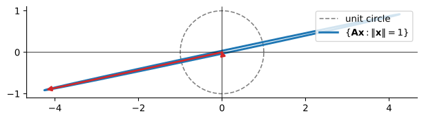
singular values: [4.349 0.035]The figure makes \sigma_1 visible as the largest distance from the origin attained by any unit vector. That observation anticipates the variational characterization below and the operator norm identity that resolves the chapter-1 definition.
The theorem, proved
Theorem (singular value decomposition). Every \mathbf{A} \in \mathbb{R}^{m \times n} admits a factorization \mathbf{A} = \mathbf{U}\boldsymbol{\Sigma}\mathbf{V}^{\mathsf T} with \mathbf{U}, \mathbf{V} orthogonal and \boldsymbol{\Sigma} diagonal with nonnegative entries. Moreover \operatorname{rank}\mathbf{A} equals the number of nonzero \sigma_i.
Proof. The matrix \mathbf{A}^{\mathsf T}\mathbf{A} \in \mathbb{R}^{n \times n} is symmetric and positive semidefinite, since \mathbf{x}^{\mathsf T}\mathbf{A}^{\mathsf T}\mathbf{A}\mathbf{x} = \lVert \mathbf{A}\mathbf{x}\rVert^2 \ge 0. By the spectral theorem (chapter 2) it diagonalizes over an orthonormal basis with nonnegative eigenvalues:
\mathbf{A}^{\mathsf T}\mathbf{A} = \mathbf{V}\operatorname{diag}(\sigma_1^2, \dots, \sigma_n^2)\mathbf{V}^{\mathsf T}, \qquad \sigma_1 \ge \cdots \ge \sigma_n \ge 0 .
Let r be the number of positive \sigma_i. For i \le r define \mathbf{u}_i = \mathbf{A}\mathbf{v}_i / \sigma_i \in \mathbb{R}^m. These are orthonormal:
\mathbf{u}_i^{\mathsf T}\mathbf{u}_j = \frac{\mathbf{v}_i^{\mathsf T}\mathbf{A}^{\mathsf T}\mathbf{A}\mathbf{v}_j}{\sigma_i\sigma_j} = \frac{\sigma_j^2\,\mathbf{v}_i^{\mathsf T}\mathbf{v}_j}{\sigma_i\sigma_j} = \delta_{ij} .
Extend \mathbf{u}_1,\dots,\mathbf{u}_r to an orthonormal basis \mathbf{u}_1,\dots,\mathbf{u}_m of \mathbb{R}^m (any orthonormal completion of the missing directions). For i > r the vector \mathbf{A}\mathbf{v}_i vanishes, because \lVert \mathbf{A}\mathbf{v}_i\rVert^2 = \mathbf{v}_i^{\mathsf T}\mathbf{A}^{\mathsf T}\mathbf{A}\mathbf{v}_i = \sigma_i^2 = 0. Hence \mathbf{A}\mathbf{v}_i = \sigma_i\mathbf{u}_i for i \le r and \mathbf{A}\mathbf{v}_i = \mathbf{0} for i > r, so
\mathbf{A} = \sum_{i=1}^r \sigma_i \mathbf{u}_i \mathbf{v}_i^{\mathsf T} = \mathbf{U}\boldsymbol{\Sigma}\mathbf{V}^{\mathsf T},
with \mathbf{U} = [\mathbf{u}_1\ \cdots\ \mathbf{u}_m], \mathbf{V} = [\mathbf{v}_1\ \cdots\ \mathbf{v}_n], and \boldsymbol{\Sigma} carrying the \sigma_i. Finally \operatorname{rank}\mathbf{A} = r: the vectors \mathbf{u}_1,\dots,\mathbf{u}_r form an orthonormal basis of the column space of \mathbf{A}, since \mathbf{A}\mathbf{v}_i = \sigma_i\mathbf{u}_i for i \le r and vanishes thereafter, so the \sigma_i\mathbf{u}_i span the same column space. \square
The proof is constructive except for the orthonormal completion of the left singular vectors — a Gram–Schmidt step, which chapter 7 makes mechanical. The only real input is the spectral theorem on \mathbf{A}^{\mathsf T}\mathbf{A}, which is why chapter 2 came first.
The variational characterization
The largest singular value has a meaning independent of the factorization: it is the operator norm, the largest stretch a matrix can inflict on a unit vector.
\sigma_1 = \lVert \mathbf{A}\rVert_2 = \max_{\lVert \mathbf{x}\rVert = 1} \lVert \mathbf{A}\mathbf{x}\rVert .
Expanding in the right singular vectors, \lVert \mathbf{A}\mathbf{x}\rVert^2 = \mathbf{x}^{\mathsf T}\mathbf{A}^{\mathsf T}\mathbf{A}\mathbf{x} = \sum_i \sigma_i^2 (\mathbf{v}_i^{\mathsf T}\mathbf{x})^2 \le \sigma_1^2 \sum_i (\mathbf{v}_i^{\mathsf T}\mathbf{x})^2 = \sigma_1^2 \lVert \mathbf{x}\rVert^2, with equality at \mathbf{x} = \mathbf{v}_1. So the supremum is \sigma_1, attained at \mathbf{v}_1. This closes the loop with chapter 1, where the operator norm was introduced abstractly: it is now identified with the top singular value. Every intermediate \sigma_k admits a similar, constrained description (the Courant–Fischer principle for rectangular matrices), but \sigma_1 and \sigma_r are the ones the course uses.
The polar decomposition
For a square \mathbf{A} \in \mathbb{R}^{n \times n} the SVD reorganizes into a single isometry times a single symmetric positive semidefinite stretch.
Polar decomposition. Every square \mathbf{A} factors as \mathbf{A} = \mathbf{Q}\mathbf{P} with \mathbf{Q} orthogonal and \mathbf{P} symmetric positive semidefinite. The factor \mathbf{P} = \sqrt{\mathbf{A}^{\mathsf T}\mathbf{A}} is unique; \mathbf{Q} is unique only when \mathbf{A} is invertible.
Existence. Write the SVD \mathbf{A} = \mathbf{U}\boldsymbol{\Sigma}\mathbf{V}^{\mathsf T} and group it as
\mathbf{A} = (\mathbf{U}\mathbf{V}^{\mathsf T})(\mathbf{V}\boldsymbol{\Sigma}\mathbf{V}^{\mathsf T}) = \mathbf{Q}\mathbf{P},
where \mathbf{Q} = \mathbf{U}\mathbf{V}^{\mathsf T} is orthogonal (a product of orthogonal matrices) and \mathbf{P} = \mathbf{V}\boldsymbol{\Sigma}\mathbf{V}^{\mathsf T} is the positive semidefinite square root of \mathbf{A}^{\mathsf T}\mathbf{A} = \mathbf{V}\boldsymbol{\Sigma}^2\mathbf{V}^{\mathsf T} constructed in chapter 2. Uniqueness of \mathbf{P}: any \mathbf{P} with \mathbf{P} \succeq 0 and \mathbf{P}^2 = \mathbf{A}^{\mathsf T}\mathbf{A} must be the principal square root, which is unique. Non-uniqueness of \mathbf{Q} when singular: along a collapsed direction (a zero singular value) one may reflect freely without changing \mathbf{A}. \square
The name is exact: a complex number factors in polar coordinates as z = r e^{i\theta} with r = \sqrt{\bar z z} \ge 0 and |e^{i\theta}| = 1; the matrix analog replaces the nonnegative modulus r by \sqrt{\mathbf{A}^{\mathsf T}\mathbf{A}} and the unit complex number e^{i\theta} by the isometry \mathbf{Q}. The decomposition separates “how much does \mathbf{A} stretch” (\mathbf{P}) from “how much does it rotate or reflect” (\mathbf{Q}).
Singular values and the Gram matrices
The two Gram matrices of \mathbf{A} share its nonzero singular values. Because \mathbf{A}^{\mathsf T}\mathbf{A}\mathbf{v}_i = \sigma_i^2\mathbf{v}_i and, symmetrically,
\mathbf{A}\mathbf{A}^{\mathsf T}\mathbf{u}_i = \mathbf{A}\frac{\mathbf{A}^{\mathsf T}\mathbf{A}\mathbf{v}_i}{\sigma_i} = \frac{\sigma_i^2 \mathbf{A}\mathbf{v}_i}{\sigma_i} = \sigma_i^2 \mathbf{u}_i,
the right singular vectors diagonalize \mathbf{A}^{\mathsf T}\mathbf{A} and the left ones diagonalize \mathbf{A}\mathbf{A}^{\mathsf T}, both with eigenvalues \sigma_i^2 (and zeros beyond r). The nonzero singular values of \mathbf{A} and \mathbf{A}^{\mathsf T} coincide. Unlike eigenvalues, singular values treat a matrix and its transpose symmetrically: both have the same ‘size’ in every singular direction.
Constructing the SVD from scratch
The proof is executable. Follow it literally: diagonalize \mathbf{A}^{\mathsf T}\mathbf{A}, take square roots for \boldsymbol{\Sigma}, and form \mathbf{U} as the normalized images \mathbf{A}\mathbf{v}_i/\sigma_i.
rng = np.random.default_rng(0)
A = rng.normal(size=(5, 4))
m, n = A.shape

lam, V = np.linalg.eigh(A.T @ A)             # spectral theorem on A^T A
order = np.argsort(-lam)                      # descending
lam, V = lam[order], V[:, order]
sigma = np.sqrt(np.maximum(lam, 0.0))        # singular values
r = int(np.sum(sigma > 1e-10))

Ur = np.zeros((m, r))
for i in range(r):
    Ur[:, i] = A @ V[:, i] / sigma[i]        # u_i = A v_i / sigma_i

Sr, Vr = np.diag(sigma[:r]), V[:, :r]
print("A == U_r Sigma_r V_r^T :", np.allclose(A, Ur @ Sr @ Vr.T))
print("U_r orthonormal        :", np.allclose(Ur.T @ Ur, np.eye(r)))
print("V  orthonormal         :", np.allclose(V.T @ V, np.eye(n)))
print("sigma_1 == ||A||_2     :", np.allclose(sigma[0], np.linalg.norm(A, 2)))
A == U_r Sigma_r V_r^T : True
U_r orthonormal : True
V orthonormal : True
sigma_1 == ||A||_2 : TrueThe compact SVD is recovered exactly from the spectral decomposition of \mathbf{A}^{\mathsf T}\mathbf{A}, and the top singular value matches the operator norm computed independently by np.linalg.norm. The only part of the proof not reproduced here is the orthonormal completion of \mathbf{U} to a full m \times m matrix, which the compact form (dropping the zero singular values and their corresponding vectors) does not need.
The condition number
The singular values quantify a matrix’s fragility. Solving \mathbf{A}\mathbf{x} = \mathbf{b} for invertible square \mathbf{A} is sensitive to the ratio of the extreme singular values.
Condition number. For invertible \mathbf{A}, define \kappa(\mathbf{A}) = \lVert \mathbf{A}\rVert_2\,\lVert \mathbf{A}^{-1}\rVert_2 = \sigma_1 / \sigma_n. Then a perturbation \delta\mathbf{b} of the right-hand side perturbs the solution by at most
\frac{\lVert \delta\mathbf{x}\rVert}{\lVert \mathbf{x}\rVert} \le \kappa(\mathbf{A})\,\frac{\lVert \delta\mathbf{b}\rVert}{\lVert \mathbf{b}\rVert} .
Proof. \mathbf{A}\delta\mathbf{x} = \delta\mathbf{b} gives \lVert \delta\mathbf{x}\rVert \le \lVert \mathbf{A}^{-1}\rVert\lVert \delta\mathbf{b}\rVert, while \lVert \mathbf{b}\rVert = \lVert \mathbf{A}\mathbf{x}\rVert \le \lVert \mathbf{A}\rVert\lVert \mathbf{x}\rVert, so \lVert \mathbf{x}\rVert^{-1} \le \lVert \mathbf{A}\rVert/\lVert \mathbf{b}\rVert. Multiplying,
\lVert \delta\mathbf{x}\rVert \le \lVert \mathbf{A}^{-1}\rVert\lVert \delta\mathbf{b}\rVert = \lVert \mathbf{A}\rVert\lVert \mathbf{A}^{-1}\rVert \cdot \frac{\lVert \delta\mathbf{b}\rVert}{\lVert \mathbf{A}\rVert} \le \kappa(\mathbf{A})\,\frac{\lVert \delta\mathbf{b}\rVert\,\lVert \mathbf{x}\rVert}{\lVert \mathbf{b}\rVert},
which rearranges to the claim. The second equality uses \lVert \mathbf{A}\rVert = \sigma_1 and \lVert \mathbf{A}^{-1}\rVert = 1/\sigma_n, since \mathbf{A}^{-1} has singular values 1/\sigma_i. \square
The bound is attained. Since \mathbf{A}^{-1}\mathbf{u}_i = \mathbf{v}_i/\sigma_i, the direction \mathbf{A}^{-1} stretches most is \mathbf{u}_n: it is mapped to \mathbf{v}_n/\sigma_n, the largest factor 1/\sigma_n. When \mathbf{x} aligns with \mathbf{v}_1 (so \lVert\mathbf{b}\rVert = \sigma_1\lVert\mathbf{x}\rVert) and \delta\mathbf{b} aligns with \mathbf{u}_n, the relative error is exactly \kappa(\mathbf{A}) times the relative input perturbation. A large condition number is the numerical meaning of “nearly singular” — the matrix inverts some directions so weakly that tiny errors in \mathbf{b} are amplified enormously in \mathbf{x}.
rng = np.random.default_rng(1)
n = 100
Q, _ = np.linalg.qr(rng.normal(size=(n, n)))
W, _ = np.linalg.qr(rng.normal(size=(n, n)))
sigma = np.geomspace(1, 1e3, n)              # sigma_1..sigma_n = 1..1000
A = Q @ np.diag(sigma) @ W.T

x = rng.normal(size=n)
b = A @ x
db = rng.normal(size=n)
db = db / np.linalg.norm(db) * np.linalg.norm(b) * 1e-4
x_tilde = np.linalg.solve(A, b + db)

rel_x = np.linalg.norm(x_tilde - x) / np.linalg.norm(x)
rel_b = np.linalg.norm(db) / np.linalg.norm(b)
print("kappa(A)              =", np.linalg.cond(A))
print("rel_x / rel_b (<= kappa):", rel_x / rel_b)
kappa(A) = 1000.0000000000107
rel_x / rel_b (<= kappa): 57.838345144508374The amplification factor \lVert \delta\mathbf{x}\rVert/\lVert \mathbf{x}\rVert divided by \lVert \delta\mathbf{b}\rVert/\lVert \mathbf{b}\rVert lands below \kappa(\mathbf{A}) = 1000, as the theorem requires; a generic random perturbation lands well below the worst case, since the worst case requires \delta\mathbf{b} to align precisely with \mathbf{u}_n, the direction that \mathbf{A}^{-1} stretches by 1/\sigma_n. The condition number is a worst-case guarantee, not a typical-case prediction — the same gap between generic and extremal behavior seen with the norm inequalities of chapter 1.
Low-rank structure and the layer perspective
The rank-one form \mathbf{A} = \sum_{i=1}^r \sigma_i \mathbf{u}_i \mathbf{v}_i^{\mathsf T} reads as a layered decomposition: the matrix is a sum of r layers, the i-th contributing \sigma_i\mathbf{u}_i\mathbf{v}_i^{\mathsf T} with weight \sigma_i. Truncating after k layers gives
\mathbf{A}_k = \sum_{i=1}^k \sigma_i \mathbf{u}_i \mathbf{v}_i^{\mathsf T}, \qquad \operatorname{rank}\mathbf{A}_k = k \quad (k \le r).
A matrix whose scree plot drops off quickly — a few dominant singular values — has its essential content in a low-dimensional subspace; everything below the knee of the plot is structure that can be discarded at small cost. Matrices with genuine low-rank signal decay fast; pure noise produces a broad spectrum that decays slowly across many layers of comparable weight.
import numpy as np
import matplotlib.pyplot as plt

rng = np.random.default_rng(0)
n = 64
xx, yy = np.meshgrid(np.linspace(-3, 3, n), np.linspace(-3, 3, n))
img = np.exp(-(xx**2 + yy**2))                # central blob
for _ in range(6):
    cx, cy = rng.uniform(-2.5, 2.5, 2)
    img += 0.7 * np.exp(-((xx - cx)**2 + (yy - cy)**2) / 0.3)
img += 0.03 * rng.normal(size=(n, n))         # faint noise

U, S, Vt = np.linalg.svd(img)
ks = [1, 3, 8, 30]
fig, axes = plt.subplots(1, len(ks), figsize=(14, 3.8))
for ax, k in zip(axes, ks):
    Ak = (U[:, :k] * S[:k]) @ Vt[:k, :]
    ax.imshow(Ak, cmap="gray", vmin=img.min(), vmax=img.max())
    ax.set_title(f"$k = {k}$", fontsize=12)
    ax.axis("off")
plt.tight_layout()
plt.show()

print("total singular values:", len(S))
print("energy in first 8 layers:", (S[:8]**2).sum() / (S**2).sum())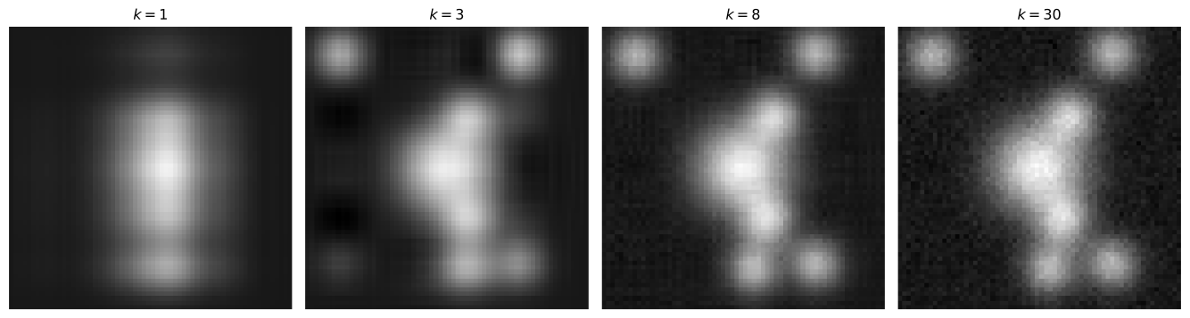
total singular values: 64
energy in first 8 layers: 0.9936763507322495
The first layer captures the dominant brightness, the next few the individual blobs, and by k = 8 essentially all the signal is present; the noise requires a long tail of small singular values. The fraction of squared Frobenius norm (energy) retained by the first k layers is \sum_{i\le k}\sigma_i^2 / \sum_i \sigma_i^2, and it rises fast when the signal is low-rank. This is the quantitative meaning of “the layers are the information”: singular values order the layers by how much of \mathbf{A} they explain.
Eckart–Young: the truncated SVD is optimal
Given the scree plot, truncating at k is the natural approximation — but is it the best rank-k approximation? The answer is the Eckart–Young theorem: nothing beats the truncated SVD.
Theorem (Eckart–Young). For any \mathbf{B} \in \mathbb{R}^{m \times n} of rank at most k, where 0 \le k < r,
\lVert \mathbf{A} - \mathbf{B}\rVert_2 \ge \lVert \mathbf{A} - \mathbf{A}_k\rVert_2 = \sigma_{k+1},
and the same holds with the Frobenius norm, where \lVert \mathbf{A} - \mathbf{A}_k\rVert_F = \big(\sum_{i > k} \sigma_i^2\big)^{1/2}. For k \ge 1 the minimizer is unique when \sigma_k > \sigma_{k+1} (k = 0 forces \mathbf{B} = \mathbf{0} outright); equal singular values at the cut admit ties.
Proof (operator norm). Since \operatorname{rank}\mathbf{B} \le k, the rank–nullity theorem (chapter 4) gives \dim \operatorname{null}\mathbf{B} \ge n - k. The subspace W = \operatorname{span}\{\mathbf{v}_1, \dots, \mathbf{v}_{k+1}\} has dimension k + 1, and
\dim \operatorname{null}\mathbf{B} + \dim W \ge (n-k) + (k+1) = n + 1 > n,
so the two subspaces intersect nontrivially. Choose a unit vector \mathbf{w} \in \operatorname{null}\mathbf{B} \cap W, written \mathbf{w} = \sum_{i=1}^{k+1} c_i \mathbf{v}_i with \sum_i c_i^2 = 1. Then
\lVert \mathbf{A} - \mathbf{B}\rVert_2^2 \ge \lVert (\mathbf{A} - \mathbf{B})\mathbf{w}\rVert^2 = \lVert \mathbf{A}\mathbf{w}\rVert^2 = \sum_{i=1}^{k+1} c_i^2 \sigma_i^2 \ge \sigma_{k+1}^2 \sum_{i=1}^{k+1} c_i^2 = \sigma_{k+1}^2,
using \mathbf{B}\mathbf{w} = \mathbf{0} in the second step and \sigma_i \ge \sigma_{k+1} in the last. Since \mathbf{A} - \mathbf{A}_k = \sum_{i > k}\sigma_i\mathbf{u}_i\mathbf{v}_i^{\mathsf T} has operator norm exactly \sigma_{k+1}, the bound is tight and \mathbf{A}_k attains it. \square
The argument has a concrete geometric reading. A rank-k matrix \mathbf{B} kills an (n-k)-dimensional subspace; among the k+1 most important directions \mathbf{v}_1,\dots,\mathbf{v}_{k+1}, some nonzero combination must fall in that kernel, and along it \mathbf{B} does nothing where \mathbf{A} stretches by at least \sigma_{k+1}. That unavoidable discrepancy is the lower bound, and \mathbf{A}_k hits it exactly.
Frobenius norm. The operator-norm argument does not carry over: the matching lower bound \lVert\mathbf{A} - \mathbf{B}\rVert_F \ge \big(\sum_{i>k}\sigma_i^2\big)^{1/2} is Mirsky’s theorem, a consequence of singular-value interlacing, not of the intersection argument above.
rng = np.random.default_rng(2)
A = rng.normal(size=(8, 6))
U, S, Vt = np.linalg.svd(A)

for k in range(5):
    Ak = (U[:, :k] * S[:k]) @ Vt[:k, :]
    err_op = np.linalg.norm(A - Ak, 2)
    err_fr = np.linalg.norm(A - Ak, "fro")
    print(f"k={k}: ||A-Ak||_2 = {err_op:.4f}   sigma_{{k+1}} = {S[k]:.4f}   "
          f"||A-Ak||_F = {err_fr:.4f}")
k=0: ||A-Ak||_2 = 4.3141 sigma_{k+1} = 4.3141 ||A-Ak||_F = 6.5786
k=1: ||A-Ak||_2 = 3.4712 sigma_{k+1} = 3.4712 ||A-Ak||_F = 4.9666
k=2: ||A-Ak||_2 = 2.3460 sigma_{k+1} = 2.3460 ||A-Ak||_F = 3.5521
k=3: ||A-Ak||_2 = 1.9331 sigma_{k+1} = 1.9331 ||A-Ak||_F = 2.6671
k=4: ||A-Ak||_2 = 1.5477 sigma_{k+1} = 1.5477 ||A-Ak||_F = 1.8376The Eckart–Young theorem converts the scree plot from a descriptive device into a guarantee: the rank-k truncation of the SVD is not merely good, it is the best possible rank-k approximation in both the operator and Frobenius norms. The two norms report the error differently: the operator norm sees the single worst direction (\sigma_{k+1}), the Frobenius norm the total tail energy \big(\sum_{i>k}\sigma_i^2\big)^{1/2}.
Summary
The SVD now packages a great deal into one factorization: the rank (number of nonzero singular values), the operator norm (\sigma_1), the condition number (\sigma_1/\sigma_n when \mathbf{A} is invertible), the best low-rank approximation (truncated SVD), the polar decomposition, and — as the proof showed — the column space of \mathbf{A}, spanned by \mathbf{u}_1,\dots,\mathbf{u}_r. The next chapter turns that last observation into a systematic account of the four fundamental subspaces: where \mathbf{A} maps, where it collapses, and how the two are related.
Problems
The problems below exercise the chapter’s definitions and theorems: the Gram matrices, the polar decomposition, the constructive proof, Eckart–Young, and the condition number as a worst-case guarantee.
[P3.1] Singular values of the Gram matrices
Let \mathbf{A} \in \mathbb{R}^{m \times n} have full SVD \mathbf{A} = \mathbf{U}\boldsymbol{\Sigma}\mathbf{V}^{\mathsf T}.
Show that the nonzero eigenvalues of \mathbf{A}^{\mathsf T}\mathbf{A} and \mathbf{A}\mathbf{A}^{\mathsf T} coincide, with the same multiplicities. Write both Gram matrices as orthogonal diagonalizations of \boldsymbol{\Sigma}^{\mathsf T}\boldsymbol{\Sigma} and \boldsymbol{\Sigma}\boldsymbol{\Sigma}^{\mathsf T}.
Conclude that \mathbf{A} and \mathbf{A}^{\mathsf T} have the same nonzero singular values, hence \lVert \mathbf{A}\rVert_2 = \lVert \mathbf{A}^{\mathsf T}\rVert_2 and, for invertible square \mathbf{A}, \kappa(\mathbf{A}) = \kappa(\mathbf{A}^{\mathsf T}).
For m > n, show that \mathbf{A}\mathbf{A}^{\mathsf T} has exactly m - n more zero eigenvalues than \mathbf{A}^{\mathsf T}\mathbf{A}.
[P3.2] The polar factor is a rotation
Let \mathbf{A} \in \mathbb{R}^{n \times n} be invertible, with SVD \mathbf{A} = \mathbf{U}\boldsymbol{\Sigma}\mathbf{V}^{\mathsf T} and polar decomposition \mathbf{A} = \mathbf{Q}\mathbf{P}.
Show that \mathbf{Q} maps right singular vectors to left singular vectors: \mathbf{Q}\mathbf{v}_i = \mathbf{u}_i for i = 1, \dots, n. Conclude that \det\mathbf{Q} = \pm 1, and that \mathbf{Q} is a rotation when \det\mathbf{A} > 0 and a reflection when \det\mathbf{A} < 0.
Show that \mathbf{Q} = \mathbf{A}(\mathbf{A}^{\mathsf T}\mathbf{A})^{-1/2}, where (\mathbf{A}^{\mathsf T}\mathbf{A})^{1/2} is the principal square root of chapter 2.
Show that the polar decomposition is unique for invertible \mathbf{A}: if \mathbf{A} = \mathbf{Q}_1\mathbf{P}_1 = \mathbf{Q}_2\mathbf{P}_2 with \mathbf{Q}_i orthogonal and \mathbf{P}_i \succeq \mathbf{0}, then \mathbf{P}_1 = \mathbf{P}_2 and \mathbf{Q}_1 = \mathbf{Q}_2.
[P3.3] The compact SVD, from the proof
The proof of the SVD theorem is constructive: diagonalize \mathbf{A}^{\mathsf T}\mathbf{A}, take square roots for the singular values, and form the left singular vectors as the normalized images \mathbf{A}\mathbf{v}_i/\sigma_i. Implement it for a rank-deficient matrix.
Let \mathbf{A} = \mathbf{B}\mathbf{C} with \mathbf{B} \in \mathbb{R}^{6 \times 3} and \mathbf{C} \in \mathbb{R}^{3 \times 5} drawn from a standard normal distribution (fixed seed), so \operatorname{rank}\mathbf{A} = 3 < \min(6, 5). The starter code computes the compact SVD of \mathbf{A} following the proof. Complete the four checks:
- The reconstruction \mathbf{U}_r\boldsymbol{\Sigma}_r\mathbf{V}_r^{\mathsf T} equals \mathbf{A}.
- \mathbf{U}_r has orthonormal columns.
- The top singular value equals the operator norm \lVert \mathbf{A}\rVert_2.
- The number of nonzero singular values equals \operatorname{rank}\mathbf{A}.
All four checks should print True. The starter code follows.
import numpy as np

rng = np.random.default_rng(7)
B = rng.normal(size=(6, 3))
C = rng.normal(size=(3, 5))
A = B @ C                                    # rank 3, shape (6, 5)

lam, V = np.linalg.eigh(A.T @ A)             # spectral theorem on A^T A
order = np.argsort(-lam)
lam, V = lam[order], V[:, order]
sigma = np.sqrt(np.maximum(lam, 0.0))
r = int(np.sum(sigma > 1e-6))                # noise floor ~1e-7, sigma_3 ~ 1.2

Ur = np.zeros((6, r))
for i in range(r):
    Ur[:, i] = A @ V[:, i] / sigma[i]        # u_i = A v_i / sigma_i

Sr, Vr = np.diag(sigma[:r]), V[:, :r]
print("singular values:", np.round(sigma, 4))

# (a) reconstruction: check A == U_r Sigma_r V_r^T
# (b) orthonormality: check U_r^T U_r == I_r
# (c) operator norm: check sigma_1 == ||A||_2
# (d) rank: check r == np.linalg.matrix_rank(A)
singular values: [6.0123 4.7448 1.1961 0. 0. ][P3.4] Eckart–Young in practice
Let \mathbf{A} \in \mathbb{R}^{8 \times 6} be drawn from a standard normal distribution (fixed seed). The starter code computes its SVD. Verify the Eckart–Young identities numerically:
- For each k = 1, \dots, 5, the truncated SVD \mathbf{A}_k = \sum_{i \le k}\sigma_i\mathbf{u}_i\mathbf{v}_i^{\mathsf T} satisfies \lVert \mathbf{A} - \mathbf{A}_k\rVert_2 = \sigma_{k+1}.
- The Frobenius error satisfies \lVert \mathbf{A} - \mathbf{A}_k\rVert_F = \big(\sum_{i > k}\sigma_i^2\big)^{1/2}.
- A random rank-3 competitor \mathbf{B} = \mathbf{X}\mathbf{Y} with \mathbf{X} \in \mathbb{R}^{8 \times 3} and \mathbf{Y} \in \mathbb{R}^{3 \times 6} cannot beat \mathbf{A}_3: verify numerically that \lVert \mathbf{A} - \mathbf{B}\rVert_2 \ge \sigma_4, which the theorem guarantees for every such \mathbf{B}.
The starter code sets up \mathbf{A} and its SVD; write the verification.
import numpy as np

rng = np.random.default_rng(11)
A = rng.normal(size=(8, 6))
U, S, Vt = np.linalg.svd(A)
print("singular values:", np.round(S, 4))

# (a) for each k = 1..5: build A_k = (U[:, :k] * S[:k]) @ Vt[:k, :] and
#     check ||A - A_k||_2 == S[k]
# (b) check ||A - A_k||_F == sqrt(sum_{i>k} S[i]**2)
# (c) a random rank-3 competitor B = X @ Y (X 8x3, Y 3x6) satisfies
#     ||A - B||_2 >= S[3]
singular values: [3.6408 3.0871 2.5967 1.863 1.5894 0.7759][P3.5] The condition number is a worst-case guarantee
Challenge. The condition-number bound of the chapter is a worst-case guarantee: generic perturbations amplify far less than \kappa(\mathbf{A}). Verify this numerically, and construct the perturbation that attains the bound.
Let \mathbf{A} \in \mathbb{R}^{100 \times 100} have singular values \sigma_i = 10^{3(n-i)/(n-1)} for i = 1, \dots, n, geometric from \sigma_1 = 1000 down to \sigma_n = 1, so \kappa(\mathbf{A}) = 1000. The starter code builds \mathbf{A} from random orthogonal factors (fixed seeds) and fixes a random \mathbf{x} with \mathbf{b} = \mathbf{A}\mathbf{x}.
- Report \kappa(\mathbf{A}) from
np.linalg.cond. - For 1000 random perturbations \delta\mathbf{b} with \lVert \delta\mathbf{b}\rVert = 10^{-4}\lVert \mathbf{b}\rVert, solve \mathbf{A}\,\delta\mathbf{x} = \delta\mathbf{b} and record the amplification factor \rho = \frac{\lVert \delta\mathbf{x}\rVert/\lVert \mathbf{x}\rVert}{\lVert \delta\mathbf{b}\rVert/\lVert \mathbf{b}\rVert}. Report the maximum and the mean; the maximum stays below \kappa(\mathbf{A}) and the mean far below.
- Worst case: take \mathbf{x} = \mathbf{v}_1, the right singular vector for \sigma_1, and \delta\mathbf{b} = 10^{-4}\lVert \mathbf{A}\mathbf{v}_1\rVert\,\mathbf{u}_n, the left singular vector for \sigma_n. Show that the amplification factor equals \kappa(\mathbf{A}) to machine precision.
- Verify that the bound \lVert \delta\mathbf{x}\rVert/\lVert \mathbf{x}\rVert \le \kappa(\mathbf{A})\,\lVert \delta\mathbf{b}\rVert/\lVert \mathbf{b}\rVert holds for every random perturbation of part (b).
The starter code follows.
import numpy as np

rng = np.random.default_rng(5)
n = 100
Q, _ = np.linalg.qr(rng.normal(size=(n, n)))
W, _ = np.linalg.qr(rng.normal(size=(n, n)))
sigma = np.geomspace(1e3, 1, n)              # sigma_1..sigma_n = 1000..1
A = Q @ np.diag(sigma) @ W.T
kappa = np.linalg.cond(A)

U, S, Vt = np.linalg.svd(A)
v1, un = Vt[0], U[:, -1]                     # v_1 and u_n

x = rng.normal(size=n)
b = A @ x
eps = 1e-4
print("kappa(A) =", kappa)

# (b) for 1000 random perturbations db with ||db|| = eps ||b||, solve
#     A dx = db and record rho = (||dx||/||x||) / (||db||/||b||);
#     report the maximum and the mean
# (c) worst case: x = v1, db = eps ||A v1|| u_n; show rho == kappa
# (d) check rho <= kappa for every random perturbation
kappa(A) = 1000.0000000000163