This chapter puts the machinery of Chapter 3 to work on a matrix built from text rather than from geometry: a collection of newsgroup messages becomes a matrix of word counts, and the low-rank factorizations developed so far turn out to recover the topics the documents discuss, without ever being told what those topics are.
The raw material is a corpus of n documents over a fixed vocabulary of d terms. The bag-of-words model discards word order and records only how often each term occurs in each document, yielding the term–document matrix\mathbf{X}\in\mathbb{R}^{n\times d} with entries
x_{ij} = \text{number of times term } j \text{ occurs in document } i,
one row per document, one column per term. All the syntax of the original texts is thrown away; what survives is a frequency table. Despite that loss, the matrix retains enough structure for the SVD to find coherent themes.
The low-rank ladder of Chapter 3 gives the motivation. The rank-one layer \sigma_1\mathbf{u}_1\mathbf{v}_1^{\mathsf T} is an outer product of a document-direction vector and a word-direction vector: it approximates every row of \mathbf{X} by a single average word-frequency profile \mathbf{v}_1, scaled per document by \sigma_1(\mathbf{u}_1)_i, a quantity proportional to the document’s length. Adding the second layer \sigma_2\mathbf{u}_2\mathbf{v}_2^{\mathsf T} superimposes a signed correction: documents with (\mathbf{u}_2)_i > 0 are pushed toward the words where (\mathbf{v}_2)_j > 0 and away from the words where (\mathbf{v}_2)_j < 0, so the layer splits the corpus into two opposing groups of documents and words: two topics. At rank k the model is
a k-topic model in which each layer is one topic and each document is a weighted combination of topics. The two factors carry the two readings: the right singular vectors \mathbf{v}_i live in word space and read as word lists; the left singular vectors \mathbf{u}_i live in document space and say how strongly each document participates in the layer.
The corpus
The data are the 20 Newsgroups collection: posts from Usenet discussion groups, restricted here to four categories: two religion-related groups (alt.atheism, talk.religion.misc), a computer-graphics group (comp.graphics), and a space group (sci.space). The category of every document is known, but the analysis below never uses it; the labels serve only as a ground-truth check after the fact. This is an unsupervised setting: the factorization must find the structure in the counts alone.
The matrix \mathbf{X}\in\mathbb{R}^{2034\times 26576} is tall and thin in the sense that matters here: d is more than an order of magnitude larger than n. The call # <1> strips message headers, footers, and quoted replies, so the counts reflect the authors’ own prose; # <2> removes a standard English stopword list; # <3> leaves a sparse matrix with 0.25% of its entries nonzero — each document uses on average only about 66 of the 26576 vocabulary terms. The labels played no role in the construction: the counts are assembled from the text alone.
The spectrum of a document matrix
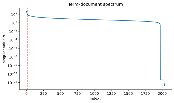
Chapter 3 established the diagnostic: the singular values of a matrix order its information content layer by layer, and the scree plot of \sigma_i against i shows how much a low-rank truncation can capture. Applied to \mathbf{X}, the same plot answers a content question first: does a document corpus actually have low-rank structure?
from scipy import linalgt0 = time.perf_counter()U, s, Vh = linalg.svd(X.todense(), full_matrices=False)t_full = time.perf_counter() - t0k =10fig, ax = plt.subplots(figsize=(7, 4.2))ax.semilogy(np.arange(1, len(s) +1), s, lw=1.6, color="#1f77b4")ax.axvline(k +0.5, color="#d62728", ls="--", lw=1.4)ax.set_xlabel("index $i$")ax.set_ylabel("singular value $\\sigma_i$")ax.set_title("Term–document spectrum")for sp in ("top", "right"): ax.spines[sp].set_visible(False)plt.tight_layout()plt.show()print(f"full SVD of dense {X.shape}: {t_full:.1f} s")print(f"energy in first {k} layers: {(s[:k]**2).sum() / (s**2).sum():.1%}")
Figure 1
full SVD of dense (2034, 26576): 62.9 s
energy in first 10 layers: 58.0%
Unlike the matrices of Chapter 3 (planted low-rank signals plus noise), the spectrum of real text decays slowly and steadily: the first ten of 2034 layers retain 58% of the total energy, and the tail keeps going far beyond the plot’s edge. Real document corpora are genuinely high-rank: the singular values fall off like a power law, not an exponential. Truncation is therefore a modeling choice: “ten topics explain 58% of the word counts”, rather than a forced recovery of a hidden low-rank truth. Chapter 3’s Eckart–Young theorem guarantees that the truncated SVD is the best rank-k approximation of \mathbf{X} in the Frobenius norm; it cannot guarantee that the best approximation is a good model. The step # <1> densifies the sparse matrix, about 430 MB of doubles, so that linalg.svd can operate on it, and the exact factorization costs 49 seconds here; both bills are what the randomized algorithms at the end of this chapter avoid.
Reading topics from the right singular vectors
Each row of \mathbf{V}^{\mathsf T} is one right singular vector \mathbf{v}_i^{\mathsf T}\in\mathbb{R}^d, with one entry per vocabulary term. The terms with the largest entries dominate the layer, and the word list they form is the topic the i-th layer captures. Because SVD entries are signed, the smallest entries are equally informative: they are the words the layer actively pulls away from, the topic’s opposite pole. The helper below extracts the n largest entries of any word-space vector; it is applied to the first ten right singular vectors.
vocab = counts.get_feature_names_out()def show_topics(a, vocab, n=8):"""Top-n vocabulary terms of a word-space vector a, largest weight first."""return [vocab[j] for j in np.argsort(a)[::-1][:n]]for i inrange(10):print(f"v_{i:2d}: "+", ".join(show_topics(Vh[i], vocab)))
The first right singular vector is an outlier: it collects rare, document-specific words (ditto, propagandist, galacticentric) that separate individual documents most sharply; the top layer does idiosyncrasy work rather than topical work. From the second layer on the vectors are unmistakably topical: \mathbf{v}_1 and \mathbf{v}_2 are computer graphics (image formats in one, graphics newsgroup slang in the other); \mathbf{v}_3 and \mathbf{v}_5 are religion and atheism; \mathbf{v}_6 and \mathbf{v}_9 are space, one about missions and probes, one about cosmology; and \mathbf{v}_8 is the argumentation register (fallacy, premises, ad argumentum), typical of the two debate-heavy groups. The category structure of the corpus was never given to the algorithm; it emerges from the counts alone, which is the punchline of the unsupervised setting.
Two structural caveats temper the reading. First, the SVD’s topics are mutually orthogonal in word space, a constraint real topics do not satisfy, so overlapping subjects bleed into neighboring layers: \mathbf{v}_4 mixes image processing with generic tools, and \mathbf{v}_7 mixes space probes with image processing. Second, each layer is signed: the words at the bottom of a vector are the layer’s opposite pole, so a layer can pair a theme with the words it opposes. Both limitations motivate the nonnegative factorization of the next section.
Nonnegative matrix factorization
The SVD’s topics are signed: a document is a linear combination of layers in which positive and negative word weights can cancel. That is numerically optimal but semantically awkward: a topic that says “astronomy, minus religion” is a subtraction, not a theme. The nonnegative matrix factorization (NMF) removes the cancellation by forcing every factor to be nonnegative:
fitting the model by minimizing \lVert \mathbf{X} - \mathbf{W}\mathbf{H}\rVert_F^2 over both factors. Each row of \mathbf{H} is a topic–word weight vector, each row of \mathbf{W} holds the k topic weights of one document, and document i is reconstructed as an additive combination of topic word lists:
Nothing is subtracted: a document is a sum of topic contributions, each one a nonnegative scaling of a single topic’s word list. That is the interpretability argument for NMF: the factors read as parts, in the same spirit as the layer view of Chapter 3, but without signed weights that demand cancellation.
NMF is not exact and not unique: no closed form exists, the objective is nonconvex, and different initializations converge to different local minima. sklearn’s implementation alternates between updating \mathbf{W} and \mathbf{H} by multiplicative updates 1 and returns one of many valid factorizations.
With k = 5 components the factorization finds the four categories: the two religion groups merge into a single topic (jesus, god, atheists covers both alt.atheism and talk.religion.misc), space gets one clean topic, and graphics splits across two near-duplicates: one about image formats (jpeg, gif, color), one about the graphics-technical register (edu, pub, ray, ftp), plus a fifth on image processing and software. The near-duplicate split is NMF’s non-uniqueness made visible: the objective has many local minima, and this run’s solver landed on one that separates graphics by register rather than merging it. Because \mathbf{W} and \mathbf{H} are nonnegative, each document is a pure additive mixture: the entry w_{ir} is literally the amount of topic r in document i, with no negative weights to interpret away — the interpretability NMF trades for exactness and uniqueness.
TF–IDF weighting
Raw counts over-reward frequent words: a term like “don” or “people” appears in most documents and dominates the reconstruction even though it carries little topical information. Term frequency–inverse document frequency (TF–IDF) reweights each count by how discriminative the term is across the corpus. For term t and document d,
\operatorname{tf}(t,d) = \frac{\text{count of } t \text{ in } d}{\text{total terms in } d},
\qquad
\operatorname{idf}(t) = \log\frac{n}{|\{d : t \in d\}|},
\qquad
\operatorname{tfidf}(t,d) = \operatorname{tf}(t,d)\cdot\operatorname{idf}(t),
so a term is heavy only if it is frequent within a document and rare across the corpus. 2 Any term appearing in nearly every document gets \operatorname{idf} \approx 0 and drops out of the reconstruction. TfidfVectorizer additionally L2-normalizes each document row, so document lengths stop dominating the fit.
The reweighting sharpens the topical cores: the space topic now reads space, nasa, launch, shuttle, orbit, moon, lunar, earth and the religion topic god, jesus, bible, believe, christian — both cleaner than their count-based counterparts, several of whose slots went to generic English (commercial, market, said). The reweighting is not free, though: the debate register that the count model folded into the religion topic (people, don, think, objective, morality) now occupies its own component, and a new topic of rare proper nouns appears: ico, bobbe, tek, beauchaine (a prolific alt.atheism correspondent), bronx, manhattan, sank, queens — the lexical fingerprint of a few long threads. TF–IDF reorders which words dominate; it does not guarantee that every component is a theme.
The reconstruction_err_ attribute reports \lVert \mathbf{X}_w - \mathbf{W}\mathbf{H}\rVert_F after fitting, a monitor of fit quality on the same matrix: 43.7 on the weighted counts against 683 on the raw counts. The two numbers are not comparable: the matrices being reconstructed differ by the weighting, and a smaller error does not mean better topics, since the factorization is non-unique and extra components can always absorb noise instead of meaning.
Truncated and randomized SVD
The full SVD above densified the matrix and paid for every one of its 2034 singular values even though only a handful were read. The exact algorithm costs \mathcal{O}(nd\cdot\min(n,d)) flops and needs the dense representation. For larger corpora (millions of documents, vocabularies in the hundreds of thousands) that is out of reach, but only k layers are wanted. The randomized SVD computes the top k singular layers directly in \mathcal{O}(ndk) flops, working on the sparse matrix, in three steps:
Sketch. Multiply \mathbf{X} by a Gaussian matrix \mathbf{G}\in\mathbb{R}^{d\times(k+p)}: the columns of \mathbf{Y}=\mathbf{X}\mathbf{G} are random linear combinations of documents.
Range finder. A QR factorization (Chapter 7) of \mathbf{Y}\in\mathbb{R}^{n\times(k+p)} produces an orthonormal \mathbf{Q} whose columns span the dominant k+p left singular subspace of \mathbf{X}.
Small SVD. The matrix \mathbf{B}=\mathbf{Q}^{\mathsf T}\mathbf{X} has only k+p rows; its exact SVD \mathbf{B}=\widehat{\mathbf{U}}\boldsymbol{\Sigma}\mathbf{V}^{\mathsf T} (Chapter 3) recovers the singular values and right singular vectors of \mathbf{X}, since \mathbf{X}\approx\mathbf{Q}\mathbf{B}.
from sklearn.utils.extmath import randomized_svdt0 = time.perf_counter()Ur, sr, Vhr = randomized_svd(X, n_components=k, random_state=1)t_rand = time.perf_counter() - t0for i inrange(k):print(f"topic {i}: "+", ".join(show_topics(Vhr[i], vocab)))print(f"randomized: {t_rand *1e3:.0f} ms full: {t_full:.1f} s")
From scratch. The same three steps, hand-rolled as a function that returns the top-k factors directly from the sparse matrix. The output compares its topics and singular values against the library call above.
def randomized_svd_scratch(A, k, n_oversamples=10, n_power=3, seed=0): rng = np.random.default_rng(seed) n, d = A.shape ell = k + n_oversamples G = rng.standard_normal((d, ell)) Y = A @ G # <1> sketchfor _ inrange(n_power): Y = A @ (A.T @ Y) # <2> power iterations Q, _ = np.linalg.qr(Y) # <3> range finder B = Q.T @ A # <4> small matrix Uhat, s, Vh = np.linalg.svd(B, full_matrices=False)return Q @ Uhat, s, VhUz, sz, Vhz = randomized_svd_scratch(X, k)for i inrange(k):print(f"topic {i}: "+", ".join(show_topics(Vhz[i], vocab)))print("singular values sklearn:", np.round(sr, 4))print("singular values scratch:", np.round(sz[:k], 4))print("|Vhr . Vhz^T| (topics up to sign):")print(np.round(np.abs(Vhr @ Vhz[:k].T), 3))
The scratch implementation reproduces the library call: the first four singular values agree to better than 10^{-5} relative error, and the overlap matrix |\mathbf{V}_r\mathbf{V}_{rz}^{\mathsf T}| is the identity up to roundoff: diagonal entries 1, off-diagonal entries below 2.4\times10^{-4}. Four of the five topic word lists agree exactly; the fifth, topic 3, is the sign-flipped twin of the library’s: its top words (space, launch, satellite, commercial) are exactly the words at the bottom of sklearn’s topic 3 (jesus, god, matthew). That is the sign ambiguity of Chapter 3 made concrete: singular vectors are determined only up to sign, and a flipped topic reads as its own anti-theme. Only the subspace spanned by the vectors is what the data determines, not the orientation of each basis vector. The fifth singular value lags by 0.05% (182.66 against 182.74): it sits in the nearly-degenerate pair \sigma_5/\sigma_6 \approx 1.09 at the edge of the retained range, where the power iterations converge most slowly, and the scratch run uses three of them where sklearn’s default uses seven.
Step # <1> samples the column space through k+p random directions, the oversampling p guarding against the slow spectrum of Figure Figure 1. The power iterations # <2> multiply the sketch by \mathbf{X}\mathbf{X}^{\mathsf T} at each pass, which squares the singular values: after q iterations the sketch is dominated by directions with \sigma_i^{2q}, exactly the amplification idea behind the power iteration of Chapter 9. The QR step # <3> turns the amplified sketch into an orthonormal basis \mathbf{Q} of the dominant subspace (Chapter 7), and the exact SVD # <4> of the (k+p)\times d matrix \mathbf{B} costs \mathcal{O}(d(k+p)^2) flops: the matrix is as wide as \mathbf{X} but has only k+p rows, so the factorization is cheap. The whole pipeline never densifies the data and never computes a singular value beyond the k wanted: 126 milliseconds against 49 seconds for the exact SVD, and the gap only widens as the corpus grows.
Summary
This chapter put the low-rank machinery of Chapter 3 on its native ground: a 2034\times 26576 term–document matrix of word counts. The SVD layers read as topics directly: the right singular vectors are word lists, and the first few recover the newsgroups’ actual subjects with no labels in sight. NMF replaces the signed layers with additive nonnegative parts, at the price of uniqueness; TF–IDF weighting sharpens the topics by downweighting corpus-wide words; and the randomized SVD computes the top layers in seconds on the sparse matrix via a Gaussian sketch, a QR range finder, and a small exact SVD: the QR of Chapter 7 and the layer view of Chapter 3, scaled to wide, sparse data.
Chapter 12 applies the same dominant-direction idea to the web: PageRank turns the link structure of the web into a matrix and finds the vector that best describes relative importance, an eigenvalue problem solved by power iteration, the Chapter 9 algorithm that resurfaces here as the range finder’s engine.
Problems
The problems exercise the machinery of this chapter: energy accounting of the SVD layers, the randomized-SVD sketch, TF–IDF weighting, and the behavior of power-law spectra. Notation follows the chapter: the term–document matrix is \mathbf{X}\in\mathbb{R}^{n\times d} with SVD \mathbf{X} = \sum_i \sigma_i\,\mathbf{u}_i\mathbf{v}_i^{\mathsf T}.
[P11.1] Energy captured by a rank-k truncation
Let \mathbf{X}\in\mathbb{R}^{n\times d} have SVD \mathbf{X} = \sum_{i=1}^{r} \sigma_i\,\mathbf{u}_i\mathbf{v}_i^{\mathsf T} and let \mathbf{X}_k = \sum_{i=1}^{k} \sigma_i\,\mathbf{u}_i\mathbf{v}_i^{\mathsf T} be its rank-k truncation, the chapter’s k-topic model.
Show that for orthonormal unit vectors \mathbf{u}, \mathbf{v} and \sigma \ge 0,
The layers \mathbf{u}_i\mathbf{v}_i^{\mathsf T} are orthogonal under the Frobenius inner product \langle \mathbf{M}, \mathbf{N}\rangle = \operatorname{tr}(\mathbf{M}^{\mathsf T}\mathbf{N}). Show this, and use it to derive \lVert \mathbf{X}_k\rVert_F^2 = \sum_{i=1}^{k}\sigma_i^2 and \lVert \mathbf{X} - \mathbf{X}_k\rVert_F^2 = \sum_{i=k+1}^{r}\sigma_i^2.
Conclude that the fraction of the Frobenius energy retained by the rank-k truncation is
and read the chapter’s newsgroups figure of 58% of the energy in the first ten layers as this ratio.
[P11.2] Power iteration amplification in the sketch
The randomized SVD of the chapter sketches the range of \mathbf{X} by \mathbf{Y} = \mathbf{X}\mathbf{G}, where \mathbf{G}\in\mathbb{R}^{d\times(k+p)} is Gaussian, and q power iterations replace the sketch by \mathbf{Y}_q = (\mathbf{X}\mathbf{X}^{\mathsf T})^q\,\mathbf{X}\mathbf{G}. Let \mathbf{X} = \mathbf{U}\boldsymbol{\Sigma}\mathbf{V}^{\mathsf T} be the reduced SVD.
Show that (\mathbf{X}\mathbf{X}^{\mathsf T})^q = \mathbf{U}\boldsymbol{\Sigma}^{2q}\mathbf{U}^{\mathsf T}, and hence \mathbf{Y}_q = \mathbf{U}\boldsymbol{\Sigma}^{2q+1}\mathbf{V}^{\mathsf T}\mathbf{G}.
Let \mathbf{g}_j be the j-th column of \mathbf{G}. Show that the component of \mathbf{Y}_q\mathbf{e}_j along the singular direction \mathbf{u}_i has magnitude \sigma_i^{2q+1}\,|\mathbf{v}_i^{\mathsf T}\mathbf{g}_j|, so the ratio of the i-th to the \ell-th direction’s content is (\sigma_i/\sigma_\ell)^{2q+1} times a ratio of random factors.
For \sigma_1 > \sigma_2 the dominant direction’s share of the sketch therefore grows like (\sigma_1/\sigma_2)^{2q+1}, up to the random factors, which are \mathcal{O}(1) with high probability. State the cost of one power iteration in terms of the nonzeros of \mathbf{X}, and explain why the chapter’s scratch run needs them: the newsgroups spectrum decays as a power law, so the gap \sigma_1/\sigma_{k+1} is small.
[P11.3] TF–IDF on a toy corpus
Four documents over the two-term vocabulary \{\text{cat}, \text{dog}\}:
Document
Text
0
cat cat cat
1
cat dog
2
dog dog dog
3
cat cat
Compute the document frequency \operatorname{df}(t), the number of documents containing term t, and the smoothed inverse document frequency of the chapter’s footnote convention,
\operatorname{idf}(t) = \log\frac{n+1}{\operatorname{df}(t)+1} + 1, \qquad n = 4,
by hand. Verify the values against the idf_ attribute of a fitted TfidfVectorizer with np.allclose(..., atol=1e-6).
Verify that every row of the vectorized matrix has unit 2-norm, the L2 normalization the chapter attributes to TfidfVectorizer.
Report the entry (1, \text{cat}), the weight of cat in document 1. Check it against the hand value \operatorname{idf}(\text{cat})/\sqrt{\operatorname{idf}(\text{cat})^2 + \operatorname{idf}(\text{dog})^2}.
The starter cell below builds the corpus and fits the vectorizer.
Implement energy_retained(s, k), the ratio \sum_{i\le k} s_i^2 / \sum_i s_i^2 for a singular-value array s, the quantity of Problem 1(c).
Build a synthetic matrix with planted singular values \sigma_i = 1/i, i = 1,\dots,40: sample orthonormal \mathbf{U}\in\mathbb{R}^{50\times 40} and \mathbf{V}\in\mathbb{R}^{40\times 40} from QR decompositions of Gaussian matrices with seed 0, and set \mathbf{A} = \mathbf{U}\operatorname{diag}(\boldsymbol{\sigma})\mathbf{V}^{\mathsf T}. Verify three properties of the function: energy_retained(s, 40) equals 1 up to roundoff; the fraction is monotone nondecreasing in k; and it matches the direct Frobenius computation \lVert \mathbf{A}_k\rVert_F^2/\lVert \mathbf{A}\rVert_F^2 of the Eckart–Young truncation to 10^{-10}.
Report the fraction for k = 10. The planted spectrum decays like the newsgroups spectrum of the chapter, whose ten-layer figure is 58%; compare the two numbers.
The starter cell below sets up the matrix and its exact SVD.
import numpy as npdef energy_retained(s, k):"""Fraction of the squared singular-value mass in the first k layers."""# return (s[:k] ** 2).sum() / (s ** 2).sum()rng = np.random.default_rng(0)n, r =50, 40sigma =1.0/ np.arange(1, r +1)U, _ = np.linalg.qr(rng.standard_normal((n, r)))V, _ = np.linalg.qr(rng.standard_normal((r, r)))A = U @ np.diag(sigma) @ V.TU, s, Vh = np.linalg.svd(A, full_matrices=False)# (b) checks, e.g. for k = 10:# Ak = U[:, :k] @ np.diag(s[:k]) @ Vh[:k, :]# direct = np.linalg.norm(Ak) ** 2 / np.linalg.norm(A) ** 2# formula = energy_retained(s, k)print("singular values s[:5]:", np.round(s[:5], 4))print("sum s^2:", round((s **2).sum(), 6))print("energy_retained(s, r) should be 1.0; fill in (a) and (b)")
singular values s[:5]: [1.     0.5    0.3333 0.25   0.2   ]
sum s^2: 1.620244
energy_retained(s, r) should be 1.0; fill in (a) and (b)
[P11.5] Power iterations in the randomized SVD
Challenge. The chapter’s scratch randomized SVD ran three power iterations on the newsgroups matrix. This problem measures what they buy, on a synthetic matrix whose spectrum decays as a power law, like the real corpus of Figure Figure 1.
Build \mathbf{A}\in\mathbb{R}^{200\times 150} with planted singular values \sigma_i = i^{-1/2}, i = 1,\dots,150: orthonormal factors from QR decompositions of Gaussian matrices with seed 3, and \mathbf{A} = \mathbf{U}\operatorname{diag}(\boldsymbol{\sigma})\mathbf{V}^{\mathsf T}.
For q \in \{0, 3, 10\} power iterations, compute a randomized top-5 SVD with p = 5 oversampling and seed 11, and measure
the worst relative error of the recovered singular values and the worst alignment of the recovered topic vectors, up to the sign ambiguity of Chapter 3.
Verify numerically that \mathrm{err}(10) < 10^{-6} while \mathrm{err}(0) > 10^{-2}, and explain the ladder through Problem 2: with \sigma_1/\sigma_6 = \sqrt{6}, the sketch’s content ratio for the sixth direction falls like (\sigma_6/\sigma_1)^{2q+1}.
Probe q = 30. The error rises again: the sketch’s component along direction 6 is proportional to \sigma_6^{2q+1}, and (\sigma_6/\sigma_1)^{61} \approx 10^{-24} sits below machine epsilon (2.2\times 10^{-16}), so the tail directions are lost to roundoff and the sketch is numerically rank-one. Confirm that \mathrm{err}(30) is large, and identify the threshold q at which (\sigma_6/\sigma_1)^{2q+1} crosses machine epsilon.
The starter cell below provides the randomized SVD and the construction.
import numpy as npdef rsvd(A, k, q, p=5, seed=11):"""Randomized top-k SVD of A with q power iterations, p oversampling.""" rng = np.random.default_rng(seed) n, d = A.shape ell = k + p G = rng.standard_normal((d, ell)) Y = A @ Gfor _ inrange(q): Y = A @ (A.T @ Y) Q, _ = np.linalg.qr(Y) B = Q.T @ A _, s_hat, Vh_hat = np.linalg.svd(B, full_matrices=False)return s_hat, Vh_hatrng = np.random.default_rng(3)n, d, k =200, 150, 5sigma =1.0/ np.sqrt(np.arange(1, d +1))U, _ = np.linalg.qr(rng.standard_normal((n, d)))V, _ = np.linalg.qr(rng.standard_normal((d, d)))A = U @ np.diag(sigma) @ V.TUe, s_exact, Vhe = np.linalg.svd(A, full_matrices=False)for q in (0, 3, 10, 30): s_hat, Vh_hat = rsvd(A, k, q)# err = np.max(np.abs(s_hat[:k] - s_exact[:k]) / s_exact[:k])# sub = np.max(1 - np.abs(np.diag(Vh_hat[:k] @ Vhe[:k].T)))print(f"q={q}: s_hat = {np.round(s_hat[:k], 4)}")
The multiplicative update rules of Lee and Seung, which multiply the current factors by entrywise nonnegative correction ratios, so nonnegativity is preserved automatically.↩︎
sklearn smooths the formula to \operatorname{idf}(t) = \log\big((n+1)/(\operatorname{df}_t+1)\big) + 1; the convention changes the scale, not the ordering of terms.↩︎