from watchtower.core import set_format
set_format("svg")Projection & orthogonalization
Projection is the geometric engine behind most of what remains in the course. Least-squares fitting (Chapter 8) is projection onto a column space; the two factors \mathbf A\mathbf A^+ and \mathbf A^+\mathbf A of the pseudoinverse (Chapter 6) are projectors. This chapter develops orthogonal projection from first principles, then turns to the computational question it raises: how to build an orthonormal basis for a subspace (Gram-Schmidt, QR) and how to exploit one.
Orthogonal projection: definition and uniqueness
Let S \subseteq \mathbb R^m be a subspace and \mathbf y \in \mathbb R^m an arbitrary vector. The orthogonal projection of \mathbf y onto S is the vector \hat{\mathbf y}\in S that makes the residual \mathbf y-\hat{\mathbf y} orthogonal to every vector of S, written \mathbf y-\hat{\mathbf y}\perp S.
Two things are not obvious and must be checked: that such a vector is unique, and that it is the closest point of S to \mathbf y. Uniqueness is a one-liner. If \hat{\mathbf y}_1,\hat{\mathbf y}_2 both satisfy the definition, then their difference is
\hat{\mathbf y}_1-\hat{\mathbf y}_2 \;\in\; S \qquad\text{and}\qquad \hat{\mathbf y}_1-\hat{\mathbf y}_2 = (\mathbf y-\hat{\mathbf y}_2)-(\mathbf y-\hat{\mathbf y}_1) \;\perp\; S .
A vector that lies both in S and in its orthogonal complement must be zero, so \hat{\mathbf y}_1=\hat{\mathbf y}_2.
Closeness follows from the Pythagorean identity. For any \mathbf s\in S, write \mathbf y-\mathbf s = (\mathbf y-\hat{\mathbf y}) + (\hat{\mathbf y}-\mathbf s). The two terms are orthogonal because \mathbf y-\hat{\mathbf y}\perp S while \hat{\mathbf y}-\mathbf s\in S, hence
\lVert\mathbf y-\mathbf s\rVert^2 = \lVert\mathbf y-\hat{\mathbf y}\rVert^2 + \lVert\hat{\mathbf y}-\mathbf s\rVert^2 \;\ge\; \lVert\mathbf y-\hat{\mathbf y}\rVert^2 .
So \hat{\mathbf y} is the nearest point of S to \mathbf y, and equality holds only at \mathbf s=\hat{\mathbf y}. Projection and best approximation are the same operation.
Projection via the SVD
Uniqueness settled, existence comes from the singular value decomposition. Let \mathbf A\in\mathbb R^{m\times n} have SVD \mathbf A = \mathbf U\boldsymbol\Sigma\mathbf V^{\mathsf T} with \operatorname{rank}\mathbf A = r. From Chapter 3, \{\mathbf u_1,\dots,\mathbf u_r\} is an orthonormal basis of \mathsf C(\mathbf A); complete it to an orthonormal basis \mathbf u_1,\dots,\mathbf u_m of \mathbb R^m. Decompose \mathbf y against this basis:
\mathbf y = \underbrace{\sum_{i=1}^{r}\mathbf u_i\mathbf u_i^{\mathsf T}\mathbf y}_{\in\,\mathsf C(\mathbf A)} + \underbrace{\sum_{i=r+1}^{m}\mathbf u_i\mathbf u_i^{\mathsf T}\mathbf y}_{\perp\,\mathsf C(\mathbf A)} .
The first sum lands in \mathsf C(\mathbf A); the second is orthogonal to it, since each \mathbf u_i with i>r is orthogonal to every \mathbf u_j with j\le r. This split is exactly the projection definition, so
\hat{\mathbf y} = \sum_{i=1}^{r}\mathbf u_i\mathbf u_i^{\mathsf T}\mathbf y = \mathbf U_r\mathbf U_r^{\mathsf T}\mathbf y .
But \mathbf U_r\mathbf U_r^{\mathsf T} = \mathbf A\mathbf A^+ by the pseudoinverse identity \mathbf A\mathbf A^+ = \mathbf U\boldsymbol\Sigma\boldsymbol\Sigma^+\mathbf U^{\mathsf T} = \mathbf U_r\mathbf U_r^{\mathsf T} from Chapter 6. The projector onto the column space is therefore
\boxed{\,P_{\mathbf A} = \mathbf A\mathbf A^+ = \mathbf U_r\mathbf U_r^{\mathsf T} = \sum_{i=1}^{r}\mathbf u_i\mathbf u_i^{\mathsf T}\,}
Projection onto \mathsf C(\mathbf A) is the sum of the first r rank-one outer products — the same pieces that assemble \mathbf A itself.
The projector matrix
The projector P = P_{\mathbf A} has a short list of structural properties, each worth internalizing.
| Property | Statement | Meaning |
|---|---|---|
| Idempotent | P^2 = P | projecting twice equals projecting once |
| Symmetric | P^{\mathsf T} = P | the projector is an orthogonal projector |
| Spectrum | eigenvalues in \{0,1\} | P\mathbf v=\mathbf v on \mathsf C(\mathbf A), P\mathbf v=\mathbf 0 on \mathsf C(\mathbf A)^{\perp} |
| Complement | \mathbf I - P projects onto \mathsf C(\mathbf A)^{\perp}=\mathsf N(\mathbf A^{\mathsf T}) | the orthogonal split \mathbf y = P\mathbf y + (\mathbf I-P)\mathbf y |
The complement is the four-subspace split of Chapter 4 in action: P is the identity on the column space and annihilates the left null space, and every \mathbf y splits uniquely into the two pieces. Idempotence alone forces the eigenvalues into \{0,1\}: if P\mathbf v = \lambda\mathbf v then \lambda\mathbf v = P\mathbf v = P^2\mathbf v = \lambda^2\mathbf v, so \lambda = \lambda^2. Symmetry adds that the two eigenspaces are orthogonal — exactly the orthogonality of the projection.
When the columns of \mathbf A are independent, \mathbf A^{\mathsf T}\mathbf A is invertible and the projector takes the familiar form P = \mathbf A(\mathbf A^{\mathsf T}\mathbf A)^{-1}\mathbf A^{\mathsf T}, with unique weights \mathbf x = (\mathbf A^{\mathsf T}\mathbf A)^{-1}\mathbf A^{\mathsf T}\mathbf y. When they are dependent, the weights are not unique, but the projection still is.
In the one-dimensional case S = \operatorname{span}\{\mathbf a\}, the formula reduces to a clean geometric statement:
P_{\mathbf a}\,\mathbf y = \mathbf a(\mathbf a^{\mathsf T}\mathbf a)^{-1}\mathbf a^{\mathsf T}\mathbf y = \lVert\mathbf y\rVert\cos\theta\;\hat{\mathbf a},
where \theta is the angle between \mathbf a and \mathbf y and \hat{\mathbf a} is the unit vector along \mathbf a. The projection is the component of \mathbf y in the direction of \mathbf a.
Projecting onto a plane. The figure below projects a test vector \mathbf b onto the column space of a random 3\times 2 matrix (a plane through the origin) and verifies that the residual is perpendicular to the plane.
import numpy as np
import matplotlib.pyplot as plt

np.random.seed(18)
A = np.random.randn(3, 2)
c = np.cross(A[:, 0], A[:, 1])      # normal to the plane C(A)
b = np.array([0.9, 0.8, 0.2])       # test vector

x = np.linalg.solve(A.T @ A, A.T @ b)   # weights via normal equations
Ax = A @ x                           # the projection

fig = plt.figure(figsize=plt.figaspect(1))
ax = fig.add_subplot(projection='3d')
xx, yy = np.meshgrid(np.linspace(-2, 2), np.linspace(-2, 2))
z = -(c[0] * xx + c[1] * yy) / c[2]
ax.plot_surface(xx, yy, z, alpha=0.4)
ax.plot([0, b[0]], [0, b[1]], [0, b[2]], 'r', label='b (test)')
ax.plot([0, Ax[0]], [0, Ax[1]], [0, Ax[2]], 'b', label='Ax (projection)')
ax.plot([Ax[0], b[0]], [Ax[1], b[1]], [Ax[2], b[2]], 'g', label='Ax - b (residual)')
ax.legend(loc='upper left', fontsize=8)
print('(Ax - b) . Ax =', (Ax - b) @ Ax)
plt.show()
(Ax - b) . Ax = 1.5178830414797062e-17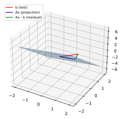
<1> The normal vector c is the cross product of the two columns, which defines the plane as \{\mathbf z : \mathbf z^{\mathsf T}c = 0\}; the surface is plotted from that equation.
<2> The weights solve the normal equations \mathbf A^{\mathsf T}\mathbf A\mathbf x = \mathbf A^{\mathsf T}\mathbf b, which is exactly \mathbf A^{\mathsf T}(\mathbf b-\mathbf A\mathbf x)=\mathbf 0 — the residual is orthogonal to both columns of \mathbf A, hence to the whole plane. The printed dot product confirms it is numerically zero.
Orthonormal columns
The factor (\mathbf A^{\mathsf T}\mathbf A)^{-1} in P = \mathbf A(\mathbf A^{\mathsf T}\mathbf A)^{-1}\mathbf A^{\mathsf T} exists only to correct for redundancy among the columns. When the columns are already orthonormal, \mathbf U^{\mathsf T}\mathbf U = \mathbf I_n, the correction is the identity, and the projector simplifies to
\boxed{\,P_{\mathbf U} = \mathbf U\mathbf U^{\mathsf T} = \sum_{j=1}^{n}\mathbf u_j\mathbf u_j^{\mathsf T}\,}
Projecting onto orthonormal directions is additive: project onto each \mathbf u_j independently and sum, with no cross-talk to remove. This is the payoff of orthonormal bases, and it motivates the next question — how to produce one from arbitrary columns.
The Gram-Schmidt process
Given columns \mathbf a_1,\dots,\mathbf a_n spanning a subspace, the Gram-Schmidt process builds an orthonormal basis \mathbf q_1,\dots,\mathbf q_r of that span one vector at a time. It is the constructive form of the projection theory above: to make \mathbf a_k orthogonal to everything already built, subtract its projection onto the span of the earlier vectors, then normalize.
- \mathbf q_1 = \mathbf a_1/\lVert\mathbf a_1\rVert.
- \mathbf q_k = \dfrac{\mathbf a_k - \sum_{j=1}^{k-1}\mathbf q_j\mathbf q_j^{\mathsf T}\mathbf a_k}{\left\lVert\mathbf a_k - \sum_{j=1}^{k-1}\mathbf q_j\mathbf q_j^{\mathsf T}\mathbf a_k\right\rVert}, for k=2,\dots,n.
The numerator \mathbf a_k - \sum_{j<k}\mathbf q_j\mathbf q_j^{\mathsf T}\mathbf a_k is \mathbf a_k with its components along \mathbf q_1,\dots,\mathbf q_{k-1} removed, so it is orthogonal to each of them; normalization then makes it a unit vector. Any column that ends up in the span of earlier columns produces a zero numerator and is discarded, which is how the process lands on exactly r vectors.
Modified Gram-Schmidt and numerical stability
Classical Gram-Schmidt has a subtle floating-point flaw. Step 2 computes every inner product \mathbf q_j^{\mathsf T}\mathbf a_k against the original \mathbf a_k, accumulating a sum of projections all at once. The modified Gram-Schmidt variant instead updates a working copy of \mathbf a_k in place, projecting away each \mathbf q_j component as soon as \mathbf q_j is formed:
- Copy \mathbf v_k = \mathbf a_k for all k.
- For k=1,\dots,n: set \mathbf q_k = \mathbf v_k/\lVert\mathbf v_k\rVert, then for j>k set \mathbf v_j \leftarrow \mathbf v_j - \mathbf q_k\mathbf q_k^{\mathsf T}\mathbf v_j.
In exact arithmetic the two are identical. In floating point they are not, and the difference is largest exactly when it matters most: columns that are nearly parallel. The next cell sweeps a parameter \varepsilon over many decades and measures how far the computed \mathbf Q is from orthonormal.
import numpy as np
import matplotlib.pyplot as plt

def cgs(A):
    U = np.zeros_like(A)
    U[:, 0] = A[:, 0] / np.linalg.norm(A[:, 0])
    for k in range(1, A.shape[1]):
        u = A[:, k] - U[:, :k] @ (U[:, :k].T @ A[:, k])   # project against originals
        U[:, k] = u / np.linalg.norm(u)
    return U

def mgs(A):
    U = np.copy(A)
    for k in range(A.shape[1]):
        U[:, k] = U[:, k] / np.linalg.norm(U[:, k])
        for j in range(k + 1, A.shape[1]):
            U[:, j] = U[:, j] - U[:, k] * (U[:, k].T @ U[:, j])   # update in place
    return U

epsilons = np.logspace(-14, -1, 14)
err_cgs, err_mgs = [], []
for eps in epsilons:
    A = np.array([[1, 1, 1], [eps, 0, 0], [0, eps, 0], [0, 0, eps]], dtype=float)
    n = A.shape[1]
    err_cgs.append(np.abs((cgs(A).T @ cgs(A)) - np.eye(n)).sum())
    err_mgs.append(np.abs((mgs(A).T @ mgs(A)) - np.eye(n)).sum())

fig, ax = plt.subplots(figsize=(6, 4))
ax.loglog(epsilons, err_cgs, 'o-', label='classical Gram-Schmidt')
ax.loglog(epsilons, err_mgs, 's-', label='modified Gram-Schmidt')
ax.set_xlabel(r'$\varepsilon$')
ax.set_ylabel(r'$\|\mathbf{Q}^{\mathsf{T}}\mathbf{Q}-\mathbf{I}\|_1$')
ax.legend()
fig.tight_layout()
plt.show()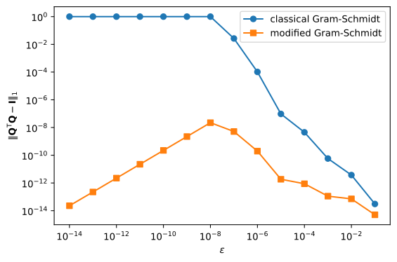
The classical variant loses orthogonality like u\kappa^2 \sim 1/\varepsilon^2 until it saturates at O(1) once \varepsilon \lesssim \sqrt{u} \approx 10^{-8}; at the smallest \varepsilon the error is total. The mechanism originates in the second column. Forming \mathbf q_2 requires the cancellation 1 - \tfrac{1}{1+\varepsilon^2} \approx \varepsilon^2 in the leading coordinate, and the rounding junk left behind, an absolute error O(u), is divided by \lVert\mathbf v_2\rVert \approx \sqrt 2\,\varepsilon during normalization: the leading coordinate of \mathbf q_2 carries a directional error of size u/\varepsilon. Classical Gram-Schmidt then forms r_{23} = \mathbf q_2^{\mathsf T}\mathbf a_3 against the original \mathbf a_3 = (1,0,0,\varepsilon). The two vectors meet only in that leading coordinate (\mathbf q_2 concentrates its mass precisely where \mathbf a_3 is supported nowhere else), so the full u/\varepsilon error flows into r_{23}, a relative blunder of order (u/\varepsilon)/\varepsilon \sim u/\varepsilon^2; the mis-sized subtraction leaves a residue of order u/\varepsilon along \mathbf q_2, which normalization by \lVert\mathbf v_3\rVert \approx \varepsilon turns into the observed \lvert\mathbf q_2^{\mathsf T}\mathbf q_3\rvert \sim u/\varepsilon^2. Modified Gram-Schmidt denies the junk any large partner: its coefficient is \mathbf q_2^{\mathsf T}\mathbf v_3 taken against the current residual, whose leading coordinate has already been cancelled down to O(\varepsilon^2), so the contaminated coordinate enters multiplied by \varepsilon^2 instead of 1 and is removed consistently in the very same subtraction. Its error stays at O(\varepsilon) across the sweep.
The QR decomposition
Gram-Schmidt is more than an algorithm for producing orthonormal bases; it is a factorization. At step k the recurrence is \mathbf a_k = \lVert\mathbf v_k\rVert\,\mathbf q_k + \sum_{j<k}(\mathbf q_j^{\mathsf T}\mathbf a_k)\mathbf q_j, so each \mathbf a_k is a combination of \mathbf q_1,\dots,\mathbf q_k only. Stacking these relations for k=1,\dots,n gives
\mathbf A = \mathbf Q\mathbf R,
where \mathbf Q has orthonormal columns and \mathbf R is upper triangular with r_{jk} = \mathbf q_j^{\mathsf T}\mathbf a_k for j\le k (and r_{jk}=0 for j>k). The QR decomposition of a full-rank matrix is unique up to signs of the diagonal of \mathbf R. NumPy computes it with Householder reflections rather than Gram-Schmidt, which keeps the orthonormality at machine precision regardless of the conditioning.
A = np.random.randn(20, 20)
Q, R = np.linalg.qr(A)
print('A - QR residual          :', np.abs(A - Q @ R).max())
print('Q^T Q - I (orthonormal)  :', np.abs(Q.T @ Q - np.eye(20)).max())
print('R is upper triangular    :', np.allclose(R, np.triu(R)))
A - QR residual : 3.774758283725532e-15
Q^T Q - I (orthonormal) : 1.1102230246251565e-15
R is upper triangular : TrueThe residual \lVert\mathbf A-\mathbf Q\mathbf R\rVert is at machine precision and \mathbf Q^{\mathsf T}\mathbf Q is exactly the identity to within roundoff — the two guarantees a QR factorization must deliver. Every entry strictly below the diagonal of \mathbf R is zero, confirming the upper-triangular structure.
Solving and inverting with QR
For a square invertible \mathbf A, the QR decomposition gives the inverse almost for free:
\boxed{\,\mathbf A^{-1} = \mathbf R^{-1}\mathbf Q^{\mathsf T}\,}
The gain is that a single system \mathbf A\mathbf x = \mathbf b costs O(n^2) once the factorization is known: solve \mathbf R\mathbf x = \mathbf Q^{\mathsf T}\mathbf b by back substitution, instead of a general O(n^3) elimination on \mathbf A. Forming \mathbf R^{-1} explicitly is still an O(n^3) operation (one back substitution per column), so the cheap path is to solve, never to invert. The next cell times both a general inverse and a triangular solve across sizes.
import time
import numpy as np
import matplotlib.pyplot as plt
from scipy.linalg import solve_triangular

inv_times, tri_times = [], []
sizes = [2**j for j in range(1, 12)]
for n in sizes:
    A = np.random.randn(n, n)
    t0 = time.perf_counter(); np.linalg.inv(A); inv_times.append(time.perf_counter() - t0)
    T = np.triu(A)
    t0 = time.perf_counter(); solve_triangular(T, np.eye(n), lower=False); tri_times.append(time.perf_counter() - t0)

fig, ax = plt.subplots(figsize=(6, 4))
ax.loglog(sizes, inv_times, 'o-', label='np.linalg.inv')
ax.loglog(sizes, tri_times, 's-', label='solve_triangular')
ax.set_xlabel(r'$n$')
ax.set_ylabel('wall time (s)')
ax.legend()
fig.tight_layout()
plt.show()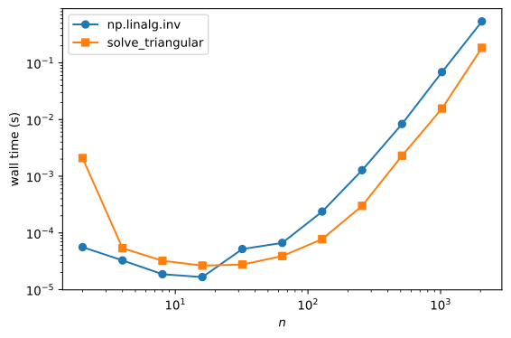
Both curves are cubic in n, but the triangular solve sits a constant factor lower — the constant that back substitution saves by never touching the zero entries. For a single linear system the right operation is solve, not an inverse at all; QR matters when the same \mathbf A is inverted against many right-hand sides, or when a triangular structure is handed to a solver that can exploit it.
The Sherman-Morrison formula
A rank-one perturbation of the identity has an explicit inverse. First note \det(\mathbf I + \mathbf u\mathbf v^{\mathsf T}) = 1 + \mathbf v^{\mathsf T}\mathbf u: expanding \det(\mathbf e_1 + v_1\mathbf u, \dots, \mathbf e_n + v_n\mathbf u) by multilinearity, the only nonzero terms are the identity term 1 and the n terms with exactly one column replaced by \mathbf u, each contributing v_j u_j — terms with two or more \mathbf u’s repeat a column and vanish. So \mathbf I+\mathbf u\mathbf v^{\mathsf T} is invertible precisely when 1+\mathbf v^{\mathsf T}\mathbf u\neq 0. In that case
\boxed{\,\left(\mathbf I + \mathbf u\mathbf v^{\mathsf T}\right)^{-1} = \mathbf I - \frac{\mathbf u\mathbf v^{\mathsf T}}{1+\mathbf v^{\mathsf T}\mathbf u}\,}
The Sherman-Morrison formula is verified by multiplying out: (\mathbf I+\mathbf u\mathbf v^{\mathsf T})(\mathbf I - \frac{\mathbf u\mathbf v^{\mathsf T}}{1+\mathbf v^{\mathsf T}\mathbf u}) telescopes to \mathbf I because the cross terms \mathbf u\mathbf v^{\mathsf T}\mathbf u\mathbf v^{\mathsf T} = (\mathbf v^{\mathsf T}\mathbf u)\,\mathbf u\mathbf v^{\mathsf T} collapse against the denominator.1
np.random.seed(1)
u = np.random.randn(5)
v = np.random.randn(5)
I = np.eye(5)
M = I + np.outer(u, v)
explicit = np.linalg.inv(M)
sherman = I - np.outer(u, v) / (1 + v @ u)
print('Sherman-Morrison residual:', np.abs(explicit - sherman).max())
Sherman-Morrison residual: 5.551115123125783e-16The formula replaces an O(n^3) inverse with O(n^2) outer products. This is the workhorse of quasi-Newton optimizers and of online linear solvers, where a solution is updated cheaply as new rank-one data arrives instead of being recomputed from scratch.
Summary
Projection onto a subspace is the unique nearest-point map, and its matrix is the sum of rank-one outer products P = \mathbf U_r\mathbf U_r^{\mathsf T} = \mathbf A\mathbf A^+ supplied directly by the SVD. The projector is idempotent and symmetric, with eigenvalues in \{0,1\} and complement \mathbf I-P on the orthogonal subspace. Gram-Schmidt turns arbitrary columns into an orthonormal basis and simultaneously yields the QR factorization \mathbf A=\mathbf Q\mathbf R; its modified variant is numerically stable where the classical one is not. QR gives cheap triangular solves via back substitution, and the Sherman-Morrison formula gives closed-form inverses for rank-one updates of the identity.
Problems
The problems below exercise the projection theory, the Gram-Schmidt process, and the Sherman-Morrison formula. Problems 1-2 are derivations, Problems 3-4 are numerical, and Problem 5 is a challenge experiment.
[P7.1] The projector and its complement
Let S\subseteq\mathbb R^m be a subspace and P the orthogonal projector onto S, so P\mathbf y\in S and \mathbf y-P\mathbf y\perp S for every \mathbf y\in\mathbb R^m.
Show that \mathbf I-P is the orthogonal projector onto S^{\perp}: it is symmetric, idempotent, and satisfies (\mathbf I-P)\mathbf y\in S^{\perp} with \mathbf y-(\mathbf I-P)\mathbf y\perp S^{\perp}.
Show that \lVert\mathbf y\rVert^2=\lVert P\mathbf y\rVert^2+\lVert(\mathbf I-P)\mathbf y\rVert^2 for every \mathbf y.
Show that \operatorname{tr}P=\dim S. Hint: the projector table’s eigenvalue argument gives the spectrum of P; the trace is the sum of the eigenvalues.
[P7.2] The closest point on a line
Let \mathbf a,\mathbf y\in\mathbb R^m with \mathbf a\neq\mathbf 0, and let S=\operatorname{span}\{\mathbf a\}.
- Expand \lVert\mathbf y-\alpha\mathbf a\rVert^2 as a quadratic in \alpha and minimize it by calculus. Show that the minimizer is \alpha^*=\mathbf a^{\mathsf T}\mathbf y/\mathbf a^{\mathsf T}\mathbf a and that the squared distance from \mathbf y to S is
\lVert\mathbf y-\alpha^*\mathbf a\rVert^2=\lVert\mathbf y\rVert^2-\frac{(\mathbf a^{\mathsf T}\mathbf y)^2}{\mathbf a^{\mathsf T}\mathbf a}.
Show that the minimizer satisfies the orthogonality condition (\mathbf y-\alpha^*\mathbf a)^{\mathsf T}\mathbf a=0, so \alpha^*\mathbf a is exactly the orthogonal projection of \mathbf y onto S.
Let \theta be the angle between \mathbf a and \mathbf y. Show that \alpha^*\lVert\mathbf a\rVert=\lVert\mathbf y\rVert\cos\theta, recovering the one-dimensional projection formula P_{\mathbf a}\mathbf y=\mathbf a(\mathbf a^{\mathsf T}\mathbf a)^{-1}\mathbf a^{\mathsf T}\mathbf y from the chapter.
[P7.3] Three routes to the projector
For a full-rank \mathbf A\in\mathbb R^{m\times n} with m>n, the projector onto \mathsf C(\mathbf A) can be built three ways: P_1=\mathbf A(\mathbf A^{\mathsf T}\mathbf A)^{-1}\mathbf A^{\mathsf T} from the normal equations, P_2=\mathbf Q\mathbf Q^{\mathsf T} from the QR decomposition, and P_3=\mathbf U_r\mathbf U_r^{\mathsf T} from the SVD. The three formulas are algebraically identical; the task is to confirm that they agree in floating point.
Compute P_1,P_2,P_3 for a random 8\times 3 matrix and a test vector \mathbf y, and report the pairwise differences \lVert P_i-P_j\rVert_1 and the idempotence residual \lVert P^2-P\rVert_1.
Verify the projection properties: the residual orthogonality \lVert(\mathbf y-P\mathbf y)^{\mathsf T}\mathbf A\rVert_\infty and the Pythagorean identity \lVert P\mathbf y\rVert^2+\lVert\mathbf y-P\mathbf y\rVert^2=\lVert\mathbf y\rVert^2.
The starter code builds the data; fill in the three projectors and the checks.
import numpy as np

rng = np.random.default_rng(7)
m, n = 8, 3
A = rng.standard_normal((m, n))
y = rng.standard_normal(m)

# P1 = A @ np.linalg.inv(A.T @ A) @ A.T          # normal equations
# P2 = Q @ Q.T                                   # from np.linalg.qr(A)
# P3 = U[:, :n] @ U[:, :n].T                     # from np.linalg.svd(A, full_matrices=False)

# (a) pairwise differences max |P_i - P_j| and idempotence residual max |P @ P - P|
# (b) residual orthogonality max |(y - P @ y) @ A| and the Pythagorean identity
[P7.4] Gram-Schmidt in floating point
The chapter’s stability demo compares classical and modified Gram-Schmidt on the matrix with columns (1,\varepsilon,0,0), (1,0,\varepsilon,0), (1,0,0,\varepsilon). This problem repeats the comparison at the fixed value \varepsilon=10^{-10} and adds the Householder QR from np.linalg.qr as a third contestant.
Implement
cgsandmgsas in the chapter, and compute the orthonormality error \lVert\mathbf Q^{\mathsf T}\mathbf Q-\mathbf I\rVert_1 for all three methods.Verify the factorization residual \lVert\mathbf A-\mathbf Q\mathbf R\rVert_\infty for all three methods. Read the result against the conditioning: with \kappa(\mathbf A)\approx\sqrt 3/\varepsilon here, backward stability only promises a residual on the order of u\,\kappa(\mathbf A) rather than machine precision, even where orthogonality itself is lost, and it is Householder QR that comes closest to working accuracy.
The starter code provides the data and the two function stubs.
import numpy as np

def cgs(A):
    """Classical Gram-Schmidt: project each column against the originals."""
    ...

def mgs(A):
    """Modified Gram-Schmidt: update a working copy in place."""
    ...

eps = 1e-10
A = np.array([[1, 1, 1], [eps, 0, 0], [0, eps, 0], [0, 0, eps]], dtype=float)
n = A.shape[1]

# (a) orthonormality error ||Q^T Q - I||_1 for cgs, mgs, and np.linalg.qr
# (b) factorization residual ||A - Q R||_inf for each
[P7.5] Sherman-Morrison: verify, invert, and break
Challenge. The Sherman-Morrison formula gives (\mathbf I+\mathbf u\mathbf v^{\mathsf T})^{-1}=\mathbf I-\mathbf u\mathbf v^{\mathsf T}/(1+\mathbf v^{\mathsf T}\mathbf u) whenever 1+\mathbf v^{\mathsf T}\mathbf u\neq 0. This experiment verifies the formula, checks the determinant identity, and probes its behavior as the matrix approaches singularity.
For n\in\{4,16,64\}, compare the formula against
np.linalg.invon random draws and report the relative error \lVert M_{\text{inv}}^{-1}-M_{\text{sm}}^{-1}\rVert_\infty/\lVert M_{\text{inv}}^{-1}\rVert_\infty. It should stay at machine precision.Verify the determinant identity \det(\mathbf I+\mathbf u\mathbf v^{\mathsf T})=1+\mathbf v^{\mathsf T}\mathbf u numerically on the same draws.
Approach singularity: fix \mathbf u, set \mathbf v=-\mathbf u/(\mathbf u^{\mathsf T}\mathbf u)+\delta\mathbf w for \delta\in\{10^{-2},10^{-7},10^{-12}\}, so that 1+\mathbf v^{\mathsf T}\mathbf u=\delta\,\mathbf w^{\mathsf T}\mathbf u shrinks with \delta. The formula is exact algebraically, but the inverse itself becomes ill-conditioned with \kappa(\mathbf I+\mathbf u\mathbf v^{\mathsf T})\approx 1/\delta. Measure the relative error and the condition number as functions of \delta, and confirm that the error grows like 1/\delta: the product of the error and \delta stays roughly constant.
The starter code sets up the draws; fill in the measurements.
import numpy as np

rng = np.random.default_rng(11)

# (a) for n in [4, 16, 64]: draw u, v; M = I + outer(u, v);
#     relative error of I - outer(u, v) / (1 + v @ u) vs np.linalg.inv(M)
for n in [4, 16, 64]:
    u = rng.standard_normal(n)
    v = rng.standard_normal(n)
    M = np.eye(n) + np.outer(u, v)
    # rel_err = ...
    # print(n, rel_err)

# (b) determinant identity: np.linalg.det(M) vs 1 + v @ u

# (c) near-singular scaling
n = 8
u = rng.standard_normal(n)
w = rng.standard_normal(n)
for delta in [1e-2, 1e-7, 1e-12]:
    v = -u / (u @ u) + delta * w
    M = np.eye(n) + np.outer(u, v)
# print(delta, 1 + v @ u, np.linalg.cond(M), rel_err)Footnotes
The Woodbury identity generalizes this to a rank-k update, (\mathbf A+\mathbf U\mathbf C\mathbf V^{\mathsf T})^{-1}, at the cost of inverting a k\times k matrix. Sherman-Morrison is its k=1 case.↩︎