The spectral theorem

Every matrix worth understanding is, at bottom, an answer to one question: in which coordinates does this linear map become transparent? For a symmetric matrix the answer is complete and beautiful. There is an orthonormal basis in which a symmetric matrix is diagonal:

\mathbf{A} = \mathbf{V}\boldsymbol{\Lambda}\mathbf{V}^{\mathsf T} = \sum_{i=1}^n \lambda_i \mathbf{v}_i \mathbf{v}_i^{\mathsf T}, \qquad \mathbf{V}^{\mathsf T}\mathbf{V} = \mathbf{I}.

The map is a pure stretch along n mutually perpendicular axes: each eigenvector \mathbf{v}_i is scaled by its eigenvalue \lambda_i and nothing else. This is the spectral theorem, the symmetric special case of the singular value decomposition. The two are equivalent and share a proof: chapter 3 obtains the SVD by running this same variational argument on the one matrix that is always symmetric, \mathbf{A}^{\mathsf T}\mathbf{A}. Most later chapters — rank, projections, least squares — lean on the factorization directly; the general eigenvalue theory of chapter 9 does not, since the SVD cannot see the eigenvalues of a nonsymmetric matrix.

The theorem deserves a complete proof, not a black box, and this chapter gives one. The route taken here avoids the fundamental theorem of algebra entirely: a real eigenvalue is produced by optimization (maximizing a quadratic form over the unit sphere), and the rest follows by restricting to a subspace and inducting. Along the way the proof manufactures the two objects that will recur throughout the course: the Rayleigh quotient and the notion of an invariant subspace.

Self-adjoint operators and symmetric matrices

Let T : \mathbb{R}^n \to \mathbb{R}^n be an operator. The adjoint of T, written T^*, is the unique operator satisfying

\langle T\mathbf{x}, \mathbf{y}\rangle = \langle \mathbf{x}, T^*\mathbf{y}\rangle \qquad\text{for all } \mathbf{x}, \mathbf{y} \in \mathbb{R}^n.

An operator is self-adjoint if T^* = T, that is, if it can slide across the inner product:

\langle T\mathbf{x}, \mathbf{y}\rangle = \langle \mathbf{x}, T\mathbf{y}\rangle .

In the standard inner product the adjoint of a matrix is its transpose, since \langle \mathbf{A}\mathbf{x}, \mathbf{y}\rangle = \mathbf{x}^{\mathsf T}\mathbf{A}^{\mathsf T}\mathbf{y} = \langle \mathbf{x}, \mathbf{A}^{\mathsf T}\mathbf{y}\rangle, so a matrix is self-adjoint exactly when it is symmetric, \mathbf{A}^{\mathsf T} = \mathbf{A}. The two notions coincide, and the course moves between them freely: symmetric for computation, self-adjoint when the argument is about the operator T itself.

Symmetric matrices are closed under sums and scalar multiples, and under transposition, but not under products: (\mathbf{A}\mathbf{B})^{\mathsf T} = \mathbf{B}^{\mathsf T}\mathbf{A}^{\mathsf T} = \mathbf{B}\mathbf{A}, so a product of symmetric matrices is symmetric precisely when they commute. The failure of closure under products is one reason the eigenvalue theory of a single symmetric matrix is so much nicer than that of a general one.

Eigenvalues and eigenvectors

A scalar \lambda \in \mathbb{R} is an eigenvalue of T if there is a nonzero vector \mathbf{v} with

T\mathbf{v} = \lambda \mathbf{v}.

The vector \mathbf{v} is an eigenvector for \lambda, and the set \{\mathbf{v} : T\mathbf{v} = \lambda\mathbf{v}\} is the eigenspace E_\lambda. For a matrix, T\mathbf{v} = \lambda\mathbf{v} is (\mathbf{A} - \lambda\mathbf{I})\mathbf{v} = \mathbf{0}, so \lambda is an eigenvalue exactly when \mathbf{A} - \lambda\mathbf{I} is singular. The polynomial p_{\mathbf{A}}(t) = \det(t\mathbf{I} - \mathbf{A}) is the characteristic polynomial, and its roots are the eigenvalues. (Some texts write \det(\mathbf{A} - t\mathbf{I}) instead; the two differ by the constant (-1)^n, so their roots coincide.) The determinant itself is defined properly in chapter 5, and the general eigenvalue theory — multiplicities, diagonalizability, nondiagonalizable matrices — is deferred to chapter 9. Here only the symmetric case is needed, and it needs no such machinery.

Two elementary facts about self-adjoint operators drive the proof, and each is worth stating separately.

Eigenvectors for distinct eigenvalues are orthogonal

Lemma. If T is self-adjoint and T\mathbf{v} = \lambda\mathbf{v}, T\mathbf{w} = \mu\mathbf{w} with \lambda \neq \mu, then \langle \mathbf{v}, \mathbf{w}\rangle = 0.

Proof. Slide T across the inner product:

\lambda\langle \mathbf{v}, \mathbf{w}\rangle = \langle T\mathbf{v}, \mathbf{w}\rangle = \langle \mathbf{v}, T\mathbf{w}\rangle = \mu\langle \mathbf{v}, \mathbf{w}\rangle .

Hence (\lambda - \mu)\langle \mathbf{v}, \mathbf{w}\rangle = 0, and since \lambda \neq \mu the inner product vanishes. \square

Distinct eigenvalues live on mutually perpendicular eigenspaces. For a repeated eigenvalue, eigenvectors are not automatically orthogonal, but the eigenspace still contains an orthonormal basis (Gram–Schmidt, chapter 7), and the theorem below shows the whole space can be assembled from orthonormal eigenspaces.

Invariant subspaces

A subspace U \subseteq \mathbb{R}^n is T-invariant if T U \subseteq U: the operator never maps a vector of U out of U. The second fact is that for a self-adjoint operator, invariance propagates to the orthogonal complement.

Lemma (invariance propagates). If T is self-adjoint and U is T-invariant, then U^\perp is also T-invariant.

Proof. Take \mathbf{w} \in U^\perp. For any \mathbf{u} \in U,

\langle T\mathbf{w}, \mathbf{u}\rangle = \langle \mathbf{w}, T\mathbf{u}\rangle = 0,

because T\mathbf{u} \in U (invariance) and \mathbf{w} is orthogonal to every vector of U. Thus T\mathbf{w} \in U^\perp. \square

This single fact is the engine of the proof: once one eigenvector is found, restriction to its orthogonal complement yields a smaller self-adjoint operator, and the problem recursively reduces by one dimension.

A real eigenvalue, by optimization

The remaining ingredient is the existence of at least one eigenvalue, and here the course departs from the usual route. Rather than appeal to the fundamental theorem of algebra, produce one directly by maximizing a quadratic form.

Lemma. A real symmetric matrix \mathbf{A} has a real eigenvalue.

Proof. The function f(\mathbf{x}) = \mathbf{x}^{\mathsf T}\mathbf{A}\mathbf{x} is continuous, and the unit sphere S^{n-1} = \{\mathbf{x} : \lVert \mathbf{x}\rVert = 1\} is compact, so f attains its maximum at some point \mathbf{x}_* \in S^{n-1}. Set \lambda_1 = f(\mathbf{x}_*).

At a constrained maximum of f subject to g(\mathbf{x}) = \mathbf{x}^{\mathsf T}\mathbf{x} = 1, the gradients are parallel: \nabla f(\mathbf{x}_*) = \mu\, \nabla g(\mathbf{x}_*). Because \mathbf{A} is symmetric, \nabla f = 2\mathbf{A}\mathbf{x} and \nabla g = 2\mathbf{x}, so \mathbf{A}\mathbf{x}_* = \mu \mathbf{x}_*: the maximizer is an eigenvector with eigenvalue \mu. Contracting with \mathbf{x}_* pins \mu down:

\mu = \mu\,\mathbf{x}_*^{\mathsf T}\mathbf{x}_* = \mathbf{x}_*^{\mathsf T}\mathbf{A}\mathbf{x}_* = \lambda_1,

which is real. \square

The proof does more than it claims: it identifies \lambda_1 as \max_{\lVert \mathbf{x}\rVert = 1} \mathbf{x}^{\mathsf T}\mathbf{A}\mathbf{x}, the largest value the quadratic form takes on the sphere. This variational reading reappears immediately below as the Rayleigh quotient principle.

The spectral theorem

Theorem (real spectral theorem). Let \mathbf{A} \in \mathbb{R}^{n \times n} be symmetric. Then \mathbb{R}^n has an orthonormal basis \mathbf{v}_1, \dots, \mathbf{v}_n of eigenvectors of \mathbf{A}. Equivalently,

\mathbf{A} = \mathbf{V}\boldsymbol{\Lambda}\mathbf{V}^{\mathsf T} = \sum_{i=1}^n \lambda_i \mathbf{v}_i \mathbf{v}_i^{\mathsf T},

where \mathbf{V} = [\mathbf{v}_1 \ \cdots \ \mathbf{v}_n] is orthogonal and \boldsymbol{\Lambda} = \operatorname{diag}(\lambda_1, \dots, \lambda_n) contains the corresponding real eigenvalues.

Proof. Induct on n. For n = 1 the claim is immediate. Suppose n \ge 2 and the result holds in dimension n-1. By the optimization lemma, choose a unit eigenvector \mathbf{v}_1 with eigenvalue \lambda_1, and let U = \operatorname{span}\{\mathbf{v}_1\}. The subspace U is invariant, so by the propagation lemma U^\perp is invariant too, and \dim U^\perp = n - 1.

The restriction of \mathbf{A} to U^\perp is again self-adjoint: the identity \langle \mathbf{A}\mathbf{x}, \mathbf{y}\rangle = \langle \mathbf{x}, \mathbf{A}\mathbf{y}\rangle holds for all \mathbf{x}, \mathbf{y} \in \mathbb{R}^n, in particular for all \mathbf{x}, \mathbf{y} \in U^\perp. By induction, U^\perp has an orthonormal basis \mathbf{v}_2, \dots, \mathbf{v}_n of eigenvectors of this restriction, hence of \mathbf{A} itself. Appending \mathbf{v}_1 yields an orthonormal basis of \mathbb{R}^n consisting of eigenvectors of \mathbf{A}, and the diagonalization

\mathbf{A} = \begin{bmatrix}\mathbf{v}_1 & \cdots & \mathbf{v}_n\end{bmatrix} \begin{bmatrix}\lambda_1 & & \\ & \ddots & \\ & & \lambda_n\end{bmatrix} \begin{bmatrix}\mathbf{v}_1^{\mathsf T} \\ \vdots \\ \mathbf{v}_n^{\mathsf T}\end{bmatrix} = \sum_{i=1}^n \lambda_i \mathbf{v}_i \mathbf{v}_i^{\mathsf T}

is immediate. \square

The rank-one form \sum_i \lambda_i \mathbf{v}_i \mathbf{v}_i^{\mathsf T} is the one that matters for computation. Each term is an outer product — a rank-one matrix (chapter 4) — so the theorem expresses \mathbf{A} as a sum of n rank-one pieces weighted by eigenvalues, exactly the outer-product view (view 4) of matrix multiplication from chapter 1. The singular value decomposition is the same idea applied to a rectangular matrix.

Immediate consequences

Reading off the diagonalization yields several identities at once.

• Trace and determinant. \operatorname{tr}(\mathbf{A}) = \sum_i \lambda_i and \det(\mathbf{A}) = \prod_i \lambda_i. Both follow because trace and determinant are invariant under the orthogonal change of basis \mathbf{A} = \mathbf{V}\boldsymbol{\Lambda}\mathbf{V}^{\mathsf T}, so \operatorname{tr}(\mathbf{A}) = \operatorname{tr}(\boldsymbol{\Lambda}) and \det(\mathbf{A}) = \det(\mathbf{V})^2\det(\boldsymbol{\Lambda}) = \det(\boldsymbol{\Lambda}).
• Invertibility. \mathbf{A} is invertible if and only if every \lambda_i \neq 0, because \mathbf{A}^{-1} = \mathbf{V}\boldsymbol{\Lambda}^{-1}\mathbf{V}^{\mathsf T}.
• Operator norm. For symmetric \mathbf{A}, the operator norm of chapter 1 is the largest absolute eigenvalue: \lVert \mathbf{A}\rVert_2 = \max_i |\lambda_i|. Write \mathbf{x} in the eigenbasis, \mathbf{x} = \sum_i c_i\mathbf{v}_i with \sum_i c_i^2 = 1; then \mathbf{A}\mathbf{x} = \sum_i \lambda_i c_i \mathbf{v}_i and \lVert \mathbf{A}\mathbf{x}\rVert^2 = \sum_i \lambda_i^2 c_i^2 \le (\max_i \lambda_i^2)\sum_i c_i^2. Equality holds at the extreme eigenvector.

The second point is the one that will matter in chapter 6: the inverse of a symmetric matrix shares its eigenvectors and inverts its eigenvalues.

The Rayleigh quotient

The optimization lemma left a loose thread worth tying. For a symmetric \mathbf{A}, the Rayleigh quotient of a nonzero vector is

R_{\mathbf{A}}(\mathbf{x}) = \frac{\mathbf{x}^{\mathsf T}\mathbf{A}\mathbf{x}}{\mathbf{x}^{\mathsf T}\mathbf{x}} .

Writing \mathbf{x} = \sum_i c_i \mathbf{v}_i in the eigenbasis gives \mathbf{x}^{\mathsf T}\mathbf{A}\mathbf{x} = \sum_i \lambda_i c_i^2 and \mathbf{x}^{\mathsf T}\mathbf{x} = \sum_i c_i^2, so R_{\mathbf{A}}(\mathbf{x}) is a weighted average of the eigenvalues, with weights c_i^2 / \sum_j c_j^2. A weighted average always lies between the extremes:

\lambda_{\min} \le R_{\mathbf{A}}(\mathbf{x}) \le \lambda_{\max} \qquad\text{for all } \mathbf{x} \neq \mathbf{0},

with equality exactly on the corresponding eigenspaces. The minimax (Courant–Fischer) formulation captures the extremes directly:¹

\lambda_{\min} = \min_{\mathbf{x} \neq \mathbf{0}} R_{\mathbf{A}}(\mathbf{x}), \qquad \lambda_{\max} = \max_{\mathbf{x} \neq \mathbf{0}} R_{\mathbf{A}}(\mathbf{x}).

The intermediate eigenvalues have a minimax description over subspaces, but the two extremes are the workhorses. They give a variational meaning to the extreme eigenvalues, and they reappear verbatim in chapter 3, where the largest singular value is \sigma_1 = \lVert \mathbf{A}\rVert_2 = \max_{\lVert \mathbf{x}\rVert = 1}\lVert \mathbf{A}\mathbf{x}\rVert, the square root of the largest eigenvalue of \mathbf{A}^{\mathsf T}\mathbf{A}.

Verification in code

The theorem is easy to verify numerically: build a random symmetric matrix, factor it with a symmetric eigensolver, and check the three claims — real eigenvalues, an orthonormal \mathbf{V}, and exact reconstruction.

from watchtower.core import set_format
set_format("svg")

import numpy as np

rng = np.random.default_rng(0)
G = rng.normal(size=(5, 5))
A = G.T @ G                                    # symmetric by construction

lam, V = np.linalg.eigh(A)                     # symmetric solver: lam sorted

print("eigenvalues real (imag part):", np.imag(lam).max())
print("max |V^T V - I|            :", np.abs(V.T @ V - np.eye(5)).max())
print("max |A - V diag(lam) V^T|  :", np.abs(A - V @ np.diag(lam) @ V.T).max())

eigenvalues real (imag part): 0.0
max |V^T V - I|            : 1.1102230246251565e-15
max |A - V diag(lam) V^T|  : 4.440892098500626e-15

np.linalg.eigh is the symmetric eigensolver, distinct from the general np.linalg.eig; it exploits symmetry to return real eigenvalues sorted in increasing order and a numerically orthogonal \mathbf{V}. The reconstruction error is on the order of machine epsilon, 10^{-15}: the spectral theorem holds to full floating-point precision, not merely approximately. This robustness is characteristic of symmetric eigenproblems, and it is the reason the SVD, built on \mathbf{A}^{\mathsf T}\mathbf{A}, inherits the same stability.

The geometry: a circle into an ellipse

The spectral theorem has a single picture. A symmetric matrix sends the unit circle to an ellipse whose principal axes are the eigenvectors and whose half-axis lengths are the eigenvalue magnitudes |\lambda_i|.

import matplotlib.pyplot as plt
import numpy as np

A = np.array([[2.0, 0.8],
              [0.8, 1.0]])                      # symmetric, PD
lam, V = np.linalg.eigh(A)

t = np.linspace(0, 2 * np.pi, 400)
circle = np.c_[np.cos(t), np.sin(t)]
image = circle @ A.T                           # map x -> A x, row-wise

fig, ax = plt.subplots(figsize=(6, 6))
ax.plot(circle[:, 0], circle[:, 1], lw=1.2, ls="--", color="gray", label="unit circle")
ax.plot(image[:, 0], image[:, 1], lw=2.0, color="#1f77b4", label=r"$\{\mathbf{A}\mathbf{x} : \|\mathbf{x}\|=1\}$")
for i in range(2):                             # eigenvector axes
    v = V[:, i] * lam[i]                       # stretched eigenvector = A v_i
    ax.annotate("", xy=v, xytext=(0, 0),
                arrowprops=dict(arrowstyle="-|>", color="#d62728", lw=2))
ax.set_aspect("equal")
ax.axhline(0, color="k", lw=0.6); ax.axvline(0, color="k", lw=0.6)
for spine in ("top", "right"): ax.spines[spine].set_visible(False)
ax.legend(fontsize=10, loc="upper right")
ax.set_title("The spectral theorem in one picture", fontsize=12)
plt.tight_layout()
plt.show()

print("eigenvalues:", lam)
print("axes (half-lengths):", np.abs(lam))
print("operator norm  ||A||_2 =", np.abs(lam).max())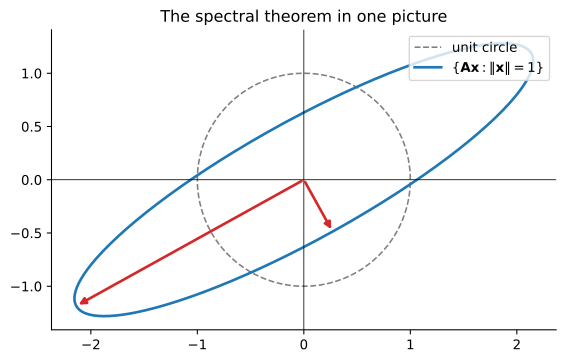

Figure 1

eigenvalues: [0.55660189 2.44339811]
axes (half-lengths): [0.55660189 2.44339811]
operator norm  ||A||_2 = 2.44339811320566

The image of the circle is \mathbf{A}\mathbf{x} as \mathbf{x} runs over the sphere, and it traces an ellipse because in the eigenbasis \mathbf{A} is a coordinate-wise stretch. The red arrows are the stretched eigenvectors \mathbf{A}\mathbf{v}_i = \lambda_i\mathbf{v}_i: they point along the axes and have length |\lambda_i|. The longer axis has length \max_i |\lambda_i|, which is precisely the operator norm — the largest stretch \mathbf{A} can inflict on a unit vector, confirming the chapter-1 definition \lVert \mathbf{A}\rVert_2 = \max_{\lVert \mathbf{x}\rVert=1}\lVert \mathbf{A}\mathbf{x}\rVert. For a symmetric matrix the operator norm and the eigenvalue of largest modulus coincide, a coincidence that breaks for nonsymmetric matrices in chapter 9.

Positive semidefinite matrices and their square roots

One further structure falls out of the spectral theorem and is needed immediately for the SVD. A symmetric matrix \mathbf{A} is positive semidefinite, written \mathbf{A} \succeq 0, if \mathbf{x}^{\mathsf T}\mathbf{A}\mathbf{x} \ge 0 for all \mathbf{x}; it is positive definite (\mathbf{A} \succ 0) if the inequality is strict for \mathbf{x} \neq \mathbf{0}.²

The eigenbasis makes the condition transparent: since \mathbf{x}^{\mathsf T}\mathbf{A}\mathbf{x} = \sum_i \lambda_i (\mathbf{v}_i^{\mathsf T}\mathbf{x})^2 and the (\mathbf{v}_i^{\mathsf T}\mathbf{x})^2 are independent nonnegative quantities, \mathbf{A} \succeq 0 if and only if \lambda_i \ge 0 for all i, and \mathbf{A} \succ 0 if and only if \lambda_i > 0 for all i. Positive semidefiniteness is a spectral property.

Positive semidefinite matrices admit square roots. Define

\mathbf{A}^{1/2} = \mathbf{V}\boldsymbol{\Lambda}^{1/2}\mathbf{V}^{\mathsf T}, \qquad \boldsymbol{\Lambda}^{1/2} = \operatorname{diag}\big(\sqrt{\lambda_1}, \dots, \sqrt{\lambda_n}\big),

the square roots being well defined because each \lambda_i \ge 0. Then \mathbf{A}^{1/2} is itself positive semidefinite and (\mathbf{A}^{1/2})^2 = \mathbf{A}. This is the principal square root, and it is unique among positive semidefinite square roots: any \mathbf{B} \succeq 0 with \mathbf{B}^2 = \mathbf{A} is simultaneously diagonalizable with \mathbf{A} and acts on each eigenspace of \mathbf{A} by the scalar \sqrt{\lambda_i}.³

The matrix that matters for the SVD is \mathbf{A}^{\mathsf T}\mathbf{A}, which is symmetric and positive semidefinite:

\mathbf{x}^{\mathsf T}\mathbf{A}^{\mathsf T}\mathbf{A}\mathbf{x} = \lVert \mathbf{A}\mathbf{x}\rVert^2 \ge 0 .

Its eigenvalues are therefore nonnegative, which is precisely why the singular values \sigma_i = \sqrt{\lambda_i(\mathbf{A}^{\mathsf T}\mathbf{A})}, the square roots of these eigenvalues, are real. The square root of \mathbf{A}^{\mathsf T}\mathbf{A}, meanwhile, is the positive factor of the polar decomposition \mathbf{A} = \mathbf{Q}\mathbf{P}, the subject of the next chapter.

rng = np.random.default_rng(2)
M = rng.normal(size=(4, 6))
G = M.T @ M                                     # symmetric PSD

lam, V = np.linalg.eigh(G)
print("min eigenvalue of A^T A :", lam.min(), " (>= 0)")

sqrt_G = V @ np.diag(np.sqrt(np.clip(lam, 0, None))) @ V.T
print("sqrt(A^T A) reconstructs :", np.allclose(sqrt_G @ sqrt_G, G))
print("sqrt(A^T A) is PSD       :", np.all(np.linalg.eigvalsh(sqrt_G) >= 0))

min eigenvalue of A^T A : -1.6930347671356328e-15  (>= 0)
sqrt(A^T A) reconstructs : True
sqrt(A^T A) is PSD       : False

The eigenvalues of \mathbf{A}^{\mathsf T}\mathbf{A} are all nonnegative, even though \mathbf{A} here is a 4 \times 6 matrix with no eigenvalues of its own (it is not square). This is the entire algebraic content of the polar decomposition: \mathbf{A}^{\mathsf T}\mathbf{A} has a symmetric positive semidefinite square root, and dividing it out of \mathbf{A} leaves an orthogonal factor.

Summary

The spectral theorem is in hand, with a complete proof and two structures the rest of the course consumes directly — the Rayleigh quotient and the positive semidefinite square root. The next step is the payoff.

Given any matrix \mathbf{A} \in \mathbb{R}^{m \times n}, the Gram matrix \mathbf{A}^{\mathsf T}\mathbf{A} is symmetric positive semidefinite, so the spectral theorem factors it as \mathbf{A}^{\mathsf T}\mathbf{A} = \mathbf{V}\operatorname{diag}(\lambda_1^2, \dots, \lambda_n^2)\mathbf{V}^{\mathsf T} with nonnegative eigenvalues \lambda_i^2 (chapter 3 renames them \sigma_i^2, the squared singular values). The chapter 3 argument then manufactures an orthogonal \mathbf{U} such that

\mathbf{A} = \mathbf{U}\boldsymbol{\Sigma}\mathbf{V}^{\mathsf T},

the singular value decomposition — the spectral theorem generalized to arbitrary matrices, symmetric or not, square or not. When \mathbf{A} is itself symmetric the two factorizations coincide, and the singular values become the absolute values of the eigenvalues, \sigma_i = |\lambda_i|.

Problems

The problems below exercise the spectral theorem, the Rayleigh quotient, and the positive semidefinite square root. Problems 1 and 2 are proofs; problems 3 and 4 are numerical verifications; problem 5 is a numerical experiment.

[P2.1] Rayleigh quotient bounds

Let \mathbf{A} \in \mathbb{R}^{n \times n} be symmetric with eigenvalues \lambda_{\min} = \lambda_1 \le \lambda_2 \le \cdots \le \lambda_n = \lambda_{\max} and an orthonormal eigenbasis \mathbf{v}_1, \dots, \mathbf{v}_n.

1. Show that for every nonzero \mathbf{x}, writing \mathbf{x} = \sum_{i=1}^n c_i \mathbf{v}_i, the Rayleigh quotient is a weighted average of the eigenvalues:

R_{\mathbf{A}}(\mathbf{x}) = \frac{\mathbf{x}^{\mathsf T}\mathbf{A}\mathbf{x}}{\mathbf{x}^{\mathsf T}\mathbf{x}} = \frac{\sum_{i=1}^n \lambda_i c_i^2}{\sum_{i=1}^n c_i^2} .

2. Conclude that \lambda_{\min} \le R_{\mathbf{A}}(\mathbf{x}) \le \lambda_{\max} for all \mathbf{x} \neq \mathbf{0}, with equality R_{\mathbf{A}}(\mathbf{x}) = \lambda_{\max} if and only if \mathbf{x} lies in the eigenspace E_{\lambda_{\max}} of the largest eigenvalue.

3. Give a short proof of the operator norm identity \lVert \mathbf{A}\rVert_2 = \max_i |\lambda_i| by applying part (b) to the symmetric matrix \mathbf{A}^2, whose eigenvalues are \lambda_i^2, and using \lVert \mathbf{A}\rVert_2^2 = \max_{\lVert \mathbf{x}\rVert = 1} \lVert \mathbf{A}\mathbf{x}\rVert^2 = \max_{\lVert \mathbf{x}\rVert = 1} \mathbf{x}^{\mathsf T}\mathbf{A}^2\mathbf{x}.

[P2.2] Uniqueness of the principal square root

Let \mathbf{A} \succeq 0 be symmetric with spectral decomposition \mathbf{A} = \mathbf{V}\boldsymbol{\Lambda}\mathbf{V}^{\mathsf T}, and let \mathbf{A}^{1/2} = \mathbf{V}\boldsymbol{\Lambda}^{1/2}\mathbf{V}^{\mathsf T} be its principal square root.

1. Show that if \mathbf{B} \succeq 0 satisfies \mathbf{B}^2 = \mathbf{A}, then \mathbf{B} commutes with \mathbf{A}, that is, \mathbf{B}\mathbf{A} = \mathbf{A}\mathbf{B}.

2. Diagonalize \mathbf{B} = \mathbf{W}\mathbf{D}\mathbf{W}^{\mathsf T} and show that \mathbf{W} is an eigenbasis of \mathbf{A}, with \mathbf{A} = \mathbf{W}\mathbf{D}^2\mathbf{W}^{\mathsf T}.

3. Conclude that \mathbf{D} = \boldsymbol{\Lambda}^{1/2} entrywise, hence \mathbf{B} = \mathbf{A}^{1/2}. Identify where the argument uses \mathbf{B} \succeq 0.

[P2.3] Verifying the spectral theorem

Build a symmetric matrix with a prescribed spectrum: take an orthogonal \mathbf{V} from the QR factorization of a random matrix and set \mathbf{A} = \mathbf{V}\operatorname{diag}(1, 2, 3, 4, 5)\mathbf{V}^{\mathsf T}. Verify numerically:

1. the eigenvalues returned by np.linalg.eigh match the prescribed ones;
2. the reconstruction \mathbf{A} = \hat{\mathbf{V}}\hat{\boldsymbol{\Lambda}}\hat{\mathbf{V}}^{\mathsf T} holds to machine precision;
3. the trace and determinant identities \operatorname{tr}(\mathbf{A}) = \sum_i \lambda_i and \det(\mathbf{A}) = \prod_i \lambda_i;
4. for a sample of random unit vectors, the Rayleigh quotient equals the weighted average \sum_i \lambda_i c_i^2 with c_i = \mathbf{v}_i^{\mathsf T}\mathbf{x}, and lies between \lambda_{\min} and \lambda_{\max}.

The starter code below sets up the matrix and the eigensolver; fill in the four checks.

import numpy as np

rng = np.random.default_rng(7)
n = 5
lam_true = np.array([1.0, 2.0, 3.0, 4.0, 5.0])

G = rng.normal(size=(n, n))
V, _ = np.linalg.qr(G)                 # orthogonal by construction
A = V @ np.diag(lam_true) @ V.T        # symmetric with prescribed spectrum

lam, Vhat = np.linalg.eigh(A)
print("computed eigenvalues:", lam)

# (a) err_lam = ...
# (b) err_recon = ...
# (c) err_tr = ...; err_det = ...
# (d) rq = ...; err_rq = ...; rq_min, rq_max = ...

computed eigenvalues: [1. 2. 3. 4. 5.]

[P2.4] The circle-to-ellipse geometry

The spectral theorem has a single picture: a symmetric matrix maps the unit circle onto an ellipse whose axes are the eigenvectors and whose half-axis lengths are the eigenvalue magnitudes. Verify this numerically for the matrix of the chapter figure,

\mathbf{A} = \begin{bmatrix} 2.0 & 0.8 \\ 0.8 & 1.0 \end{bmatrix} .

1. Sample the unit circle densely and compute the image \{\mathbf{A}\mathbf{x} : \lVert \mathbf{x}\rVert = 1\}. Show that the largest and smallest distances from the origin over the sampled image equal the half-axis lengths |\lambda_{\max}| and |\lambda_{\min}|.

2. Show that the direction of the farthest image point is the eigenvector of \lambda_{\max} up to sign, and that the residual \lVert \mathbf{A}\mathbf{v}_i - \lambda_i \mathbf{v}_i\rVert vanishes for both eigenvectors.

The starter code below samples the circle and computes the image; fill in the three checks.

import numpy as np

A = np.array([[2.0, 0.8],
              [0.8, 1.0]])             # symmetric, PD (chapter figure)

lam, V = np.linalg.eigh(A)

t = np.linspace(0, 2 * np.pi, 20000)
circle = np.c_[np.cos(t), np.sin(t)]
image = circle @ A.T                   # map x -> A x, row-wise

# (a) dist = ...; d_max, d_min = ...
# (b) farthest direction vs eigenvector of lam.max(); residual = ...

[P2.5] Power iteration and the Rayleigh quotient

Challenge. Let \mathbf{A} be symmetric with eigenvalues ordered \lambda_1 > \lambda_2 \ge \cdots \ge \lambda_n, so that \lambda_1 = \lambda_{\max}, and let \mathbf{v}_1 be a unit eigenvector for \lambda_1. The power iteration is the sequence of normalized iterates \mathbf{x}_{k+1} = \mathbf{A}\mathbf{x}_k / \lVert \mathbf{A}\mathbf{x}_k\rVert.

1. Write \mathbf{x}_0 = \sum_i c_i \mathbf{v}_i in the eigenbasis and show that if c_1 \neq 0, then \mathbf{x}_k \to \pm \mathbf{v}_1 and R_{\mathbf{A}}(\mathbf{x}_k) \to \lambda_1. Show further that the error decays geometrically,

|R_{\mathbf{A}}(\mathbf{x}_k) - \lambda_1| = O\!\left(\left(\frac{\lambda_2}{\lambda_1}\right)^{2k}\right),

where \lambda_2 denotes the eigenvalue of second-largest modulus. The gap \lambda_1 - \lambda_2 controls the convergence rate.

2. Implement power iteration for \mathbf{A}_1 = \mathbf{V}\operatorname{diag}(3, 1, 0)\mathbf{V}^{\mathsf T} with a fixed-seed orthogonal \mathbf{V}. Measure the error e_k = |R_{\mathbf{A}_1}(\mathbf{x}_k) - 3| for k = 0, \dots, 30 and verify that the ratio e_{k+1}/e_k approaches (\lambda_2/\lambda_1)^2 = 1/9.

3. Repeat with \mathbf{A}_2 = \mathbf{V}\operatorname{diag}(3, 2.9, 0)\mathbf{V}^{\mathsf T}. Verify that the ratio now approaches (2.9/3)^2 \approx 0.934 and that after 30 iterations the error remains far above machine precision: the smaller gap slows convergence.

4. Verify the operator norm identity \lVert \mathbf{A}\rVert_2 = \max_i |\lambda_i| for both matrices, and confirm that the operator norm is 3 in both cases.

The starter code below sets up both matrices and the iteration; fill in the ratio and error measurements.

import numpy as np

rng = np.random.default_rng(23)

def power_iteration(A, x0, k):
    x = x0 / np.linalg.norm(x0)
    rqs = np.empty(k)
    for i in range(k):
        x = A @ x
        x = x / np.linalg.norm(x)
        rqs[i] = x @ A @ x
    return rqs

G = rng.normal(size=(3, 3))
V, _ = np.linalg.qr(G)
x0 = rng.normal(size=3)

A1 = V @ np.diag([3.0, 1.0, 0.0]) @ V.T
A2 = V @ np.diag([3.0, 2.9, 0.0]) @ V.T

rq1 = power_iteration(A1, x0, 30)
rq2 = power_iteration(A2, x0, 30)

# (b) err1 = ...; ratio1 = ...
# (c) err2 = ...; ratio2 = ...
# (d) norm1 = ...; norm2 = ...

Footnotes

1. Named for Richard Courant and Ernst Fischer; Hermann Weyl proved the related perturbation bound (chapter 9) that makes symmetric eigenvalue problems numerically tame.

2. “Definite” here attaches to the quadratic form \mathbf{x}^{\mathsf T}\mathbf{A}\mathbf{x}, studied for its own sake in chapter 10, where the geometric meaning of \succ 0 (a bowl, not a saddle) is examined.

3. Uniqueness: diagonalize \mathbf{B} = \mathbf{W}\mathbf{D}\mathbf{W}^{\mathsf T}; then \mathbf{A} = \mathbf{B}^2 = \mathbf{W}\mathbf{D}^2\mathbf{W}^{\mathsf T}, so \mathbf{W} is an eigenbasis of \mathbf{A} and \mathbf{D}^2 = \boldsymbol{\Lambda}, forcing \mathbf{D} = \boldsymbol{\Lambda}^{1/2} entrywise. Where an eigenvalue repeats, the vectors inside its eigenspace are not pinned down, but the action is still multiplication by \sqrt{\lambda_i}, so the square root is unaffected.