from watchtower.core import set_format
set_format("svg")Eigendecomposition
The spectral theorem of Chapter 2 settles the story for symmetric matrices: every symmetric matrix admits an orthonormal basis of real eigenvectors. A general square matrix enjoys no such guarantee, and two genuinely new phenomena appear. First, eigenvalues may be complex, even for a matrix with real entries. Second, the eigenvectors may fail to span the whole space, so the matrix cannot be diagonalized at all. This chapter develops the theory that handles both.
Three facts anchor everything that follows. The eigenvalues are exactly the roots of a single degree-n polynomial, the characteristic polynomial; they can be located without solving anything through Gershgorin’s circle theorem; and, when a matrix is diagonalizable, its powers, trace, and determinant all reduce to scalars. The chapter closes with the power method, the simplest algorithm for finding the dominant eigenvalue, which is the computational engine behind PageRank.
Eigenvalues and eigenvectors
A nonzero vector \mathbf{v} is an eigenvector of \mathbf{A}\in\mathbb{R}^{n\times n} when the action of \mathbf{A} on it is pure scaling:
\mathbf{A}\mathbf{v} = \lambda\mathbf{v}.
The scalar \lambda is the corresponding eigenvalue. The defining equation says that on the line spanned by \mathbf{v}, the linear map \mathbf{A} acts as multiplication by \lambda — the direction is preserved, only the length changes.
Two immediate observations. First, \lambda is an eigenvalue exactly when \lambda\mathbf{I} - \mathbf{A} fails to be invertible, because that failure is equivalent to the existence of a nonzero \mathbf{v} with (\lambda\mathbf{I}-\mathbf{A})\mathbf{v}=\mathbf{0}. Second, \lambda = 0 is an eigenvalue precisely when \mathbf{A} has a nontrivial null space, i.e. \mathbf{A} is singular.
Eigenvectors for a given eigenvalue are not unique: any nonzero scalar multiple is again an eigenvector, and the set of all of them (together with \mathbf{0}) forms a subspace.
Existence and the characteristic polynomial
Whether \lambda\mathbf{I}-\mathbf{A} is invertible is decided by its determinant. Define the characteristic polynomial
p_{\mathbf{A}}(\lambda) = \det(\lambda\mathbf{I} - \mathbf{A}).
Expanding the determinant shows p_{\mathbf{A}} is a monic polynomial of degree n in \lambda. Since a matrix is singular exactly when its determinant vanishes, \lambda is an eigenvalue of \mathbf{A} if and only if p_{\mathbf{A}}(\lambda)=0.
The fundamental theorem of algebra factors p_{\mathbf{A}} over \mathbb{C}:
p_{\mathbf{A}}(\lambda) = \prod_{i=1}^{s} (\lambda - \lambda_i)^{r_i}, \qquad r_1 + \cdots + r_s = n,
where \lambda_1,\dots,\lambda_s are the distinct eigenvalues. The exponent r_i is the algebraic multiplicity of \lambda_i. A real matrix therefore has exactly n eigenvalues counted with multiplicity, though they may be complex; and it has at most n distinct ones.
Gershgorin’s circle theorem
The eigenvalues are the roots of a degree-n polynomial, which in general cannot be found in closed form. But they can be localized cheaply. For each row i, define the Gershgorin disk
D_i = \Big\{\, z\in\mathbb{C} : |z - a_{ii}| \le r_i \,\Big\}, \qquad r_i = \sum_{j \ne i} |a_{ij}|,
centered at the diagonal entry a_{ii} with radius equal to the sum of the off-diagonal moduli in row i.
Gershgorin’s circle theorem. Every eigenvalue of \mathbf{A} lies in the union D_{\mathbf{A}} = \bigcup_{i=1}^n D_i of the Gershgorin disks.
To see why, take an eigenpair \mathbf{A}\mathbf{v}=\lambda\mathbf{v} and choose an index i with |v_i| = \max_j |v_j| = \lVert\mathbf{v}\rVert_\infty. The i-th component of the equation reads
(\lambda - a_{ii}) v_i = \sum_{j\ne i} a_{ij} v_j,
so, dividing by v_i and taking moduli,
|\lambda - a_{ii}| \le \sum_{j\ne i} |a_{ij}|\, \frac{|v_j|}{|v_i|} \le \sum_{j\ne i} |a_{ij}| = r_i.
Thus \lambda \in D_i. The theorem is a one-line bound with real teeth: it certifies, for instance, that a strictly diagonally dominant matrix (one with |a_{ii}| > r_i for every i) has no zero eigenvalue, hence is invertible.
Note
The disks are drawn from row sums, but the column sums give an identical bound, since \mathbf{A} and \mathbf{A}^{\mathsf T} share eigenvalues.
import numpy as np
import matplotlib.pyplot as plt

A = np.array([[2.0, -1.0,  0.0],
              [1.0,  4.0, -1.0],
              [-1.0, -1.0, -3.0]])

fig, ax = plt.subplots(figsize=(5.2, 5.2))
for i in range(A.shape[0]):
    center = A[i, i]
    radius = np.sum(np.abs(A[i, :])) - abs(A[i, i])
    ax.add_patch(plt.Circle((center, 0), radius,
                            fill=False, ec='k', ls='--', lw=1))

eigs = np.linalg.eigvals(A)
ax.scatter(eigs.real, eigs.imag, marker='x', s=70, color='r', zorder=3)
ax.axhline(0, color='gray', lw=0.5); ax.axvline(0, color='gray', lw=0.5)
ax.set_aspect('equal'); ax.set_xlabel('Re'); ax.set_ylabel('Im')
ax.grid(True, alpha=0.3); fig.tight_layout()

print('eigenvalues:', np.round(eigs, 3))
eigenvalues: [ 3.162+0.j 3. +0.j -3.162+0.j]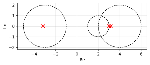
Gershgorin localization.
Each eigenvalue (red cross) lies inside the union of the three disks, as the theorem guarantees. Here the disks overlap, but the localization is already informative: the spectrum is confined to [-5, 6], and the disk at a_{33}=-3 of radius 2 isolates a single eigenvalue in the left half-plane.
The theorem generalizes: a similarity transform \mathbf{A}\mapsto \mathbf{D}\mathbf{A}\mathbf{D}^{-1} with positive diagonal \mathbf{D} preserves the spectrum while rescaling the off-diagonal entries, and a clever choice of \mathbf{D} can shrink the localization arbitrarily.
Diagonalization
A matrix is diagonalizable when it possesses n linearly independent eigenvectors. Collect them as the columns of \mathbf{V} and the eigenvalues as \boldsymbol{\Lambda}=\operatorname{diag}(\lambda_1,\dots,\lambda_n); the eigen-equations \mathbf{A}\mathbf{v}_i = \lambda_i\mathbf{v}_i assemble into \mathbf{A}\mathbf{V} = \mathbf{V}\boldsymbol{\Lambda}, and since \mathbf{V} is invertible,
\boxed{\;\mathbf{A} = \mathbf{V}\boldsymbol{\Lambda}\mathbf{V}^{-1}.\;}
In the eigenbasis the map is diagonal: it stretches coordinate i by \lambda_i and mixes nothing. Powers collapse to scalars,
\mathbf{A}^k = \mathbf{V}\boldsymbol{\Lambda}^k\mathbf{V}^{-1},
which is the reason diagonalization matters for any iterated dynamics.
One subtlety worth recording. Expanding \mathbf{A}=\mathbf{V}\boldsymbol{\Lambda}\mathbf{V}^{-1} as a sum of rank-one terms gives
\mathbf{A} = \sum_{i=1}^{n} \lambda_i\, \mathbf{v}_i \mathbf{w}_i^{\mathsf T},
where \mathbf{w}_i^{\mathsf T} is the i-th row of \mathbf{V}^{-1}, i.e. the left eigenvector \mathbf{A}^{\mathsf T}\mathbf{w}_i = \lambda_i \mathbf{w}_i. The two families are biorthogonal, \mathbf{w}_i^{\mathsf T}\mathbf{v}_j = \delta_{ij}. Only when \mathbf{A} is symmetric (Chapter 2) do the two coincide, \mathbf{w}_i = \mathbf{v}_i, collapsing this to the spectral theorem’s \mathbf{A}=\sum_i\lambda_i\mathbf{v}_i\mathbf{v}_i^{\mathsf T}.
import numpy as np

rng = np.random.default_rng(1)
A = rng.standard_normal((4, 4))

lam, V = np.linalg.eig(A)
# reconstruct A = V Lambda V^{-1}
recon = (V @ np.diag(lam)) @ np.linalg.inv(V)
print('max |A - V Lambda V^{-1}| =', np.max(np.abs(A - recon)))

# powers collapse: A^5 = V Lambda^5 V^{-1}
k = 5
err_pow = np.max(np.abs(np.linalg.matrix_power(A, k) - (V @ np.diag(lam**k)) @ np.linalg.inv(V)))
print(f'max |A^5 - V Lambda^5 V^{-1}| = {err_pow:.2e}')

# left eigenvectors: rows of V^{-1} are biorthogonal to the columns of V
W = np.linalg.inv(V)
print('max |W V - I|              =', np.max(np.abs(W @ V - np.eye(4))))
print('max |A^T W^T - W^T Lambda| =', np.max(np.abs(A.T @ W.T - W.T @ np.diag(lam))))
max |A - V Lambda V^{-1}| = 1.44349424796038e-15
max |A^5 - V Lambda^5 V^-1| = 1.60e-14
max |W V - I| = 2.222087621814296e-16
max |A^T W^T - W^T Lambda| = 1.3325180118266506e-15The reconstruction and the power identity both hold to machine precision, and the two final checks confirm that the rows of \mathbf{W}=\mathbf{V}^{-1} are left eigenvectors. The diagonalization is exact for this generic matrix, and that is the point: generic matrices are diagonalizable, and the failure is a measure-zero, structurally special event.
When diagonalization fails
Not every matrix is diagonalizable. Consider
\mathbf{A} = \begin{bmatrix} 1 & 0 \\ 1 & 1 \end{bmatrix}.
Its characteristic polynomial is (1-\lambda)^2, so \lambda=1 has algebraic multiplicity 2. But the eigen-equation (\mathbf{A}-\mathbf{I})\mathbf{v}=\mathbf{0} is
\begin{bmatrix} 0 & 0 \\ 1 & 0 \end{bmatrix}\begin{bmatrix} v_1 \\ v_2 \end{bmatrix} = \mathbf{0} \quad\Longrightarrow\quad v_1 = 0,
so every eigenvector is a multiple of [0,\ 1]^{\mathsf T}. The eigenspace is one-dimensional, and \mathbf{A} has no second independent eigenvector — it cannot be diagonalized. Such a matrix is called defective, and its structure is a Jordan block rather than a diagonal of scalars.
import numpy as np

A = np.array([[1.0, 0.0],
              [1.0, 1.0]])

lam, V = np.linalg.eig(A)
print('eigenvalues :', lam)
print('rank of V   :', np.linalg.matrix_rank(V), '(needs 2 to diagonalize)')

# try to reconstruct: V is singular so A = V Lambda V^{-1} is impossible
print('det(V)      :', np.linalg.det(V))
eigenvalues : [1.+0.j 1.+0.j]
rank of V : 1 (needs 2 to diagonalize)
det(V) : (-2.2204460492503185e-16+0j)NumPy reports the two (equal) eigenvalues, but the eigenvector matrix \mathbf{V} has rank 1 — a numerical smoking gun for defectiveness. The matrix still has a perfectly good theory (the Jordan form), but it is not of the tidy diagonal kind, and its powers grow polynomially rather than geometrically: \mathbf{A}^k = \begin{bmatrix}1&0\\ k&1\end{bmatrix}.
Geometric multiplicity is bounded by algebraic multiplicity
The eigenspace of \lambda is E_\lambda = \operatorname{N}(\lambda\mathbf{I}-\mathbf{A}), and its dimension is the geometric multiplicity of \lambda. The geometric multiplicity counts independent eigenvectors; the algebraic multiplicity counts how many times \lambda is a root of p_{\mathbf{A}}. The two need not agree — the defective matrix above has algebraic multiplicity 2 but geometric multiplicity 1 — but they are ordered.
Proposition. For every eigenvalue, geometric multiplicity \le algebraic multiplicity.
Let k = \dim E_\lambda and extend a basis \mathbf{v}_1,\dots,\mathbf{v}_k of E_\lambda to a basis of \mathbb{R}^n, collected as columns of an invertible \mathbf{V}. Since each \mathbf{v}_i is a \lambda-eigenvector,
\mathbf{A}\mathbf{V} = \mathbf{V}\begin{bmatrix} \lambda \mathbf{I}_k & \mathbf{C} \\ \mathbf{0} & \mathbf{D} \end{bmatrix},
so \mathbf{A} is similar to that block-upper-triangular matrix. The characteristic polynomial is invariant under similarity, and the determinant of a block-triangular matrix is the product of the block determinants:
p_{\mathbf{A}}(\mu) = \det(\mu\mathbf{I}-\mathbf{A}) = \det\big((\mu-\lambda)\mathbf{I}_k\big)\,\det(\mu\mathbf{I}_{n-k}-\mathbf{D}) = (\mu-\lambda)^k \det(\mu\mathbf{I}_{n-k}-\mathbf{D}).
Hence (\mu-\lambda)^k divides p_{\mathbf{A}}(\mu), so the algebraic multiplicity of \lambda is at least k. In particular, \mathbf{A} is diagonalizable exactly when every eigenvalue has geometric multiplicity equal to its algebraic multiplicity.
Eigenspaces are invariant subspaces
An eigenspace is the simplest kind of invariant subspace: \mathbf{A} maps E_\lambda into itself, since \mathbf{A}\mathbf{v}=\lambda\mathbf{v}\in E_\lambda. This constrains the geometry of a matrix. Consider
\mathbf{B} = \begin{bmatrix} 0 & 1 & 0 \\ -1 & 0 & 0 \\ 0 & 0 & -5 \end{bmatrix},
a rotation by \pi/2 in the xy-plane combined with scaling by -5 along the z-axis. The xy-plane is a two-dimensional invariant subspace, but the restriction of \mathbf{B} to it is a rotation, which has no real eigenvectors (no real vector is mapped to a scalar multiple of itself by a 90^\circ rotation). Hence \mathbf{B} has no real eigendecomposition; its eigenvalues are \pm i and -5. This is the generic picture for real matrices with complex eigenvalues: they rotate inside a real invariant plane.
Triangular matrices
For an upper- or lower-triangular matrix, the eigenvalues are the diagonal entries. The reason is that \mu\mathbf{I}-\mathbf{A} remains triangular with diagonal \mu-a_{11},\dots,\mu-a_{nn}, and the determinant of a triangular matrix is the product of its diagonal entries:
p_{\mathbf{A}}(\mu) = \prod_{i=1}^n (\mu - a_{ii}).
Schur’s theorem says every square matrix is unitarily similar to an upper-triangular one (its Schur form), and the QR algorithm realizes exactly this reduction by orthogonal similarity transformations, which is why an O(n^3) algorithm suffices to compute the full spectrum.
Trace and determinant
Two scalar invariants of \mathbf{A} are determined by its eigenvalues, whether or not \mathbf{A} is diagonalizable:
\boxed{\;\det\mathbf{A} = \prod_{i=1}^n \lambda_i, \qquad \operatorname{tr}\mathbf{A} = \sum_{i=1}^n \lambda_i.\;}
Both follow from matching coefficients of p_{\mathbf{A}}(\mu)=\prod_i(\mu-\lambda_i). For the determinant, evaluate at \mu=0:
p_{\mathbf{A}}(0) = \det(-\mathbf{A}) = (-1)^n\det\mathbf{A} = \prod_i (-\lambda_i) = (-1)^n\prod_i \lambda_i,
so \det\mathbf{A}=\prod_i\lambda_i. For the trace, the coefficient of \mu^{n-1} in \det(\mu\mathbf{I}-\mathbf{A}) is -\sum_i a_{ii} = -\operatorname{tr}\mathbf{A}, because a term contributing \mu^{n-1} picks n-1 diagonal factors \mu and one diagonal entry -a_{ii}. Matching against -\sum_i\lambda_i from the factored form gives \operatorname{tr}\mathbf{A}=\sum_i\lambda_i.
import numpy as np

rng = np.random.default_rng(3)
A = rng.standard_normal((5, 5))
lam = np.linalg.eigvals(A)

print('det(A)        =', np.linalg.det(A))
print('prod(eigvals) =', np.prod(lam))
print('tr(A)         =', np.trace(A))
print('sum(eigvals)  =', np.sum(lam))
det(A) = 1.8269058625543482
prod(eigvals) = (1.8269058625543453-4.273745946688848e-17j)
tr(A) = 0.5145653024486103
sum(eigvals) = (0.5145653024486097+0j)Both identities hold even though \mathbf{A} is a generic non-symmetric matrix with complex eigenvalues. The trace identity explains a useful shortcut: for any square matrix, \operatorname{tr}(\mathbf{A}^{\mathsf T}\mathbf{A}) = \sum_i \sigma_i^2 = \lVert\mathbf{A}\rVert_{\mathrm{F}}^2, connecting the Frobenius norm of Chapter 1 to the singular values of Chapter 3.
Complex eigenvalues come in conjugate pairs
For a real matrix, the complex eigenvalues occur in conjugate pairs. Taking the complex conjugate of \mathbf{A}\mathbf{v}=\lambda\mathbf{v} gives \mathbf{A}\bar{\mathbf{v}}=\bar{\lambda}\bar{\mathbf{v}} (since \mathbf{A} is real, \bar{\mathbf{A}}=\mathbf{A}), so \bar{\lambda} is an eigenvalue with eigenvector \bar{\mathbf{v}}. This is why \det\mathbf{A}=\prod_i\lambda_i is real even when individual \lambda_i are complex, and why a real matrix of odd order always has at least one real eigenvalue: the complex eigenvalues pair up, leaving an odd count to be real.
The power method
Suppose \mathbf{A} is diagonalizable with a dominant eigenvalue, |\lambda_1| > |\lambda_2| \ge \cdots \ge |\lambda_n|. Write an arbitrary starting vector \mathbf{x}_0 in the eigenbasis, \mathbf{x}_0 = \sum_i c_i\mathbf{v}_i with c_1\ne 0. Iterating \mathbf{x}_{k+1}=\mathbf{A}\mathbf{x}_k,
\mathbf{x}_k = \mathbf{A}^k\mathbf{x}_0 = \lambda_1^k\left( c_1\mathbf{v}_1 + \sum_{i\ge 2} c_i\left(\frac{\lambda_i}{\lambda_1}\right)^{k}\mathbf{v}_i\right),
and every term with i\ge 2 decays like |\lambda_i/\lambda_1|^k. The iterates align with \mathbf{v}_1 at rate |\lambda_2/\lambda_1|, and the Rayleigh quotient of Chapter 2 converges to \lambda_1:
\frac{\mathbf{x}_k^{\mathsf T}\mathbf{A}\mathbf{x}_k}{\mathbf{x}_k^{\mathsf T}\mathbf{x}_k} \longrightarrow \lambda_1.
Normalizing at each step keeps \mathbf{x}_k from overflowing or underflowing, giving the power method:
\mathbf{x}_{k+1} = \frac{\mathbf{A}\mathbf{x}_k}{\lVert\mathbf{A}\mathbf{x}_k\rVert_2}, \qquad \mu_k = \mathbf{x}_k^{\mathsf T}\mathbf{A}\mathbf{x}_k.
This is the algorithm behind PageRank: the web’s link structure forms a sparse matrix, and its dominant eigenvector (found by the power method) ranks pages. The method’s virtue is that it needs only matrix-vector products, never a factorization.
import numpy as np
import matplotlib.pyplot as plt

rng = np.random.default_rng(0)
B = rng.standard_normal((6, 6))
A = (B + B.T) / 2

lam = np.linalg.eigvalsh(A)
lam1 = lam[np.argmax(np.abs(lam))]
lam2 = lam[np.argsort(-np.abs(lam))[1]]

x = rng.standard_normal(6)
x /= np.linalg.norm(x)
mu = []
for k in range(1, 201):
    x = A @ x
    x /= np.linalg.norm(x)
    mu.append(x @ A @ x)

fig, ax = plt.subplots(figsize=(6, 3.6))
ax.plot(range(1, 201), mu, marker='o', ms=2, lw=0.8, label='Rayleigh quotient')
ax.axhline(lam1, color='r', ls='--', lw=1, label=rf'$\lambda_1$ = {lam1:.4f}')
ax.set_xlabel('iteration $k$'); ax.set_ylabel(r'$\mu_k$')
ax.legend(); fig.tight_layout()

print(f'lambda_1 = {lam1:.6f},  |lambda_2/lambda_1| = {abs(lam2/lam1):.3f}')
print(f'mu_200   = {mu[-1]:.6f}')
lambda_1 = -2.003712, |lambda_2/lambda_1| = 0.906
mu_200 = -2.003712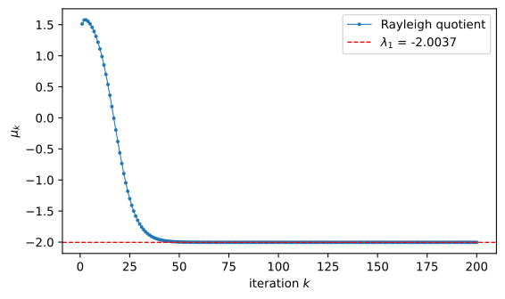
Power method convergence.
<1>A symmetric matrix keeps the eigenvalues real and the eigenvectors orthogonal, the cleanest setting for the method.<2>Ground-truth eigenvalues for comparison, computed by a dense solver.<3>Renormalization is what distinguishes the power method from raw iteration of \mathbf{A}^k; it prevents overflow and keeps the vector a unit vector.<4>The Rayleigh quotient \mu_k = \mathbf{x}_k^{\mathsf T}\mathbf{A}\mathbf{x}_k converges to \lambda_1 faster than the vector \mathbf{x}_k itself.
The quotient converges to \lambda_1, but slowly, because the printed ratio |\lambda_2/\lambda_1|=0.906 is close to 1: the eigenvector error decays by only a factor 0.906 per step. The Rayleigh quotient compensates with quadratic convergence, its error shrinking like |\lambda_2/\lambda_1|^{2k}, so a couple hundred iterations still pin \lambda_1 to six decimals. A well-separated dominant eigenvalue converges in a handful of steps; here the gap is deliberately narrow to make the rate visible. The one failure mode is a tie, |\lambda_1|=|\lambda_2|, for instance a dominant complex conjugate pair: the iterates then oscillate between the two directions instead of settling, and the plain power method must be replaced by a subspace (block) variant.
How much do eigenvalues move? Weyl’s bound
Data matrices are perturbed matrices: measurements carry noise, rounding leaves residue, and what a solver actually diagonalizes is \mathbf{A}+\mathbf{E} rather than \mathbf{A}. For symmetric matrices the answer is clean. Weyl’s inequality: if \rho(\mathbf{E}) = \lVert\mathbf{E}\rVert_2, then for every k
\boxed{\lvert\lambda_k(\mathbf{A}+\mathbf{E}) - \lambda_k(\mathbf{A})\rvert \le \rho(\mathbf{E}).}
Each eigenvalue moves by at most the size of the perturbation, in absolute terms, no matter how the eigenvectors are arranged. The proof is two applications of the Courant-Fischer characterization from chapter 2, \lambda_k(\mathbf{M}) = \max_{\dim\mathcal{S}=k}\ \min_{\substack{\mathbf{x}\in\mathcal{S}\\ \lVert\mathbf{x}\rVert=1}}\mathbf{x}^{\mathsf T}\mathbf{M}\mathbf{x}. Since |\mathbf{x}^{\mathsf T}\mathbf{E}\mathbf{x}| \le \rho(\mathbf{E}) for every unit \mathbf{x},
\lambda_k(\mathbf{A}+\mathbf{E}) = \max_{\dim\mathcal{S}=k}\min_{\mathbf{x}}\big(\mathbf{x}^{\mathsf T}\mathbf{A}\mathbf{x} + \mathbf{x}^{\mathsf T}\mathbf{E}\mathbf{x}\big) \;\ge\; \max_{\dim\mathcal{S}=k}\Big(\min_{\mathbf{x}}\mathbf{x}^{\mathsf T}\mathbf{A}\mathbf{x} - \rho(\mathbf{E})\Big) = \lambda_k(\mathbf{A}) - \rho(\mathbf{E}),
and swapping the roles of \mathbf{A} and \mathbf{A}+\mathbf{E} gives the matching upper bound. When \mathbf{A}+\mathbf{E} is normal as well, more is true in aggregate: the Hoffman-Wielandt inequality matches the eigenvalues pairwise as \sum_i\lvert\mu_i-\lambda_i\rvert^2 \le \lVert\mathbf{E}\rVert_{\mathrm F}^2.
Eigenvalues are perfectly conditioned; eigenvectors are not. Let \lambda_1 > \lambda_2 \ge \dots be the eigenvalues of symmetric \mathbf{A} with gap \gamma = \lambda_1 - \lambda_2, and let (\mu, \mathbf{w}) be an eigenpair of \mathbf{A}+\mathbf{E} with \mu near \lambda_1. The residual obeys \mathbf{r} = (\mathbf{A}-\mu\mathbf{I})\mathbf{w} = -\mathbf{E}\mathbf{w}, so \lVert\mathbf{r}\rVert \le \rho(\mathbf{E}). Expanding \mathbf{w} = \sum_i c_i\mathbf{u}_i in the eigenbasis of \mathbf{A},
\lVert\mathbf{r}\rVert^2 = \sum_i c_i^2(\lambda_i-\mu)^2 \;\ge\; (\gamma - \rho(\mathbf{E}))^2 \sum_{i\ge 2} c_i^2,
because every old eigenvalue except \lambda_1 lies at distance at least \gamma - \rho(\mathbf{E}) from \mu: Weyl pins \mu within \rho(\mathbf{E}) of \lambda_1, while \lambda_i \le \lambda_1 - \gamma for i \ge 2. The sum on the right is exactly the squared distance from \mathbf{w} to the line spanned by \mathbf{u}_1, which for unit vectors is \sin^2\theta, the sine of the angle between them. Provided \rho(\mathbf{E}) \le \gamma/2,
\boxed{\sin\theta(\mathbf{w}, \mathbf{u}_1) \;\le\; \frac{2\,\rho(\mathbf{E})}{\lambda_1 - \lambda_2}.}
This is the simplest case of the Davis-Kahan \sin\theta theorem; the general version bounds the angles between invariant subspaces by the perturbation norm divided by the spectral gap surrounding them. The message for practice: eigenvalue error is absolute, eigenvector error scales like the inverse gap. A perturbation of size 10^{-3} is invisible in the spectrum of a matrix whose top eigenvalues differ by O(1), yet it can rotate a pair split by 10^{-3} through angles of order one.
Numerical check. Same perturbation norm, two spectra: one with a healthy top gap, one with the top two eigenvalues nearly tied.
import numpy as np

def top_eigenpair_experiment(lam_desc, e_norm):
    n = len(lam_desc)
    rng = np.random.default_rng(7)
    Q, _ = np.linalg.qr(rng.standard_normal((n, n)))
    A = Q @ np.diag(np.sort(lam_desc)) @ Q.T            # symmetric with the given spectrum
    u1, u2 = Q[:, -1], Q[:, -2]
    F = e_norm * (np.outer(u1, u2) + np.outer(u2, u1))  # ||F||_2 = e_norm, aimed at the top pair
    mu, W = np.linalg.eigh(A + F)
    w1 = W[:, -1]
    if u1 @ w1 < 0:
        w1 = -w1
    sin_theta = np.sqrt(max(0.0, 1.0 - (u1 @ w1) ** 2))
    return abs(mu[-1] - lam_desc[0]), sin_theta

e_norm = 5e-3
scenarios = {
    'well-separated (gap 1)':   np.concatenate([[10.0, 9.0], np.linspace(-8.0, 0.0, 38)]),
    'clustered top (gap 1e-3)': np.concatenate([[10.0, 10.0 - 1e-3], np.linspace(-8.0, 0.0, 38)]),
}
for name, lam in scenarios.items():
    dlam, st = top_eigenpair_experiment(lam, e_norm)
    print(f'{name}:  |dlam_1|={dlam:.2e} (bound {e_norm:.0e}),  '
          f'sin(theta)={st:.2e} (bound {min(1.0, 2 * e_norm / (lam[0] - lam[1])):.2f})')
well-separated (gap 1): |dlam_1|=2.50e-05 (bound 5e-03), sin(theta)=5.00e-03 (bound 0.01)
clustered top (gap 1e-3): |dlam_1|=4.52e-03 (bound 5e-03), sin(theta)=6.71e-01 (bound 1.00)The experiment confirms the split personality: the top eigenvalue moves by at most \rho(\mathbf{E}) in both scenarios, while the top eigenvector stays put only when the gap is generous. When spectra cluster, individual eigenvectors are meaningful only through the subspace they span, which is why practical algorithms (and chapter 13) target subspaces rather than single directions whenever the gap is thin.
Summary
The eigendecomposition generalizes the spectral theorem at the cost of two complications: complex eigenvalues and defective matrices. The eigenvalues are the roots of the characteristic polynomial, localized by Gershgorin disks and read off directly for triangular matrices; the trace and determinant are their sum and product. When n independent eigenvectors exist the matrix diagonalizes, \mathbf{A}=\mathbf{V}\boldsymbol{\Lambda}\mathbf{V}^{-1}, and iterated dynamics reduce to scalar powers. When they do not, the matrix is defective and the Jordan form takes over. The power method turns the dominant-eigenvalue theory into an algorithm needing only matrix-vector products — the bridge from this chapter’s theory to the least-squares optimization of Chapter 8 and the quadratic forms of Chapter 10.
Problems
The problems below exercise the chapter’s main results: Gershgorin localization, diagonalizability, defective matrices, and the power method. Problems 1 and 2 are theory; Problems 3 and 4 are computational; Problem 5 is a numerical experiment.
[P9.1] Strict diagonal dominance implies invertibility
Let \mathbf{A}\in\mathbb{R}^{n\times n} be strictly diagonally dominant: |a_{ii}| > r_i for every i, where r_i = \sum_{j\ne i}|a_{ij}| is the radius of the i-th Gershgorin disk D_i.
- Show that 0 lies outside every disk D_i.
- Conclude from Gershgorin’s circle theorem that \mathbf{A} is invertible.
- Suppose in addition that a_{ii} > 0 for every i. Show that every eigenvalue of \mathbf{A} has positive real part. [Hint: locate the disks in the complex plane.]
[P9.2] Distinct eigenvalues imply diagonalizability
Let \mathbf{A}\in\mathbb{R}^{n\times n} have n distinct eigenvalues \lambda_1,\dots,\lambda_n.
- Show that each eigenvalue has geometric multiplicity at least 1.
- Combine (a) with the proposition that geometric multiplicity is bounded above by algebraic multiplicity to show that each eigenvalue has geometric multiplicity exactly 1.
- Conclude that \mathbf{A} is diagonalizable.
[P9.3] Verifying Gershgorin’s theorem and its scaling refinement
- For the fixed random matrix \mathbf{A} below, verify that every eigenvalue lies in at least one Gershgorin disk: the quantity
\max_i \min_j \big(|\lambda_i - a_{jj}| - r_j\big)
should be nonpositive.
Verify that the similarity transform \mathbf{B} = \mathbf{D}\mathbf{A}\mathbf{D}^{-1} with \mathbf{D} = \operatorname{diag}(1,2,3,4,5) preserves the spectrum: \max_i|\lambda_i(\mathbf{B}) - \lambda_i(\mathbf{A})| should be at machine precision.
For \mathbf{M} = \begin{bmatrix}1 & 100\\ 0.001 & 1\end{bmatrix}, the first row gives a disk of radius 100, and the union of the two disks has diameter 200. Apply the scaling \mathbf{D} = \operatorname{diag}(1, 1000) and show that the union of disks of \mathbf{D}\mathbf{M}\mathbf{D}^{-1} has diameter 2, while the spectrum is unchanged.
The starter code below provides the disk helper and the data; the three parts are left to be completed.
import numpy as np

def gershgorin_disks(M):
    centers = np.diag(M)
    radii = np.sum(np.abs(M), axis=1) - np.abs(np.diag(M))
    return centers, radii

rng = np.random.default_rng(7)
A = rng.standard_normal((5, 5))
eigs = np.linalg.eigvals(A)
print('eigenvalues of A:', np.round(eigs, 3))

# (a) max over eigenvalues of min_j(|lambda - a_jj| - r_j); should be <= 0
# violation = ...

# (b) B = D A D^{-1} with D = diag(1, 2, 3, 4, 5); compare eigenvalues
# D = ...
# B = ...

# (c) union diameter of M before and after D = diag(1, 1000)
# M = ...
eigenvalues of A: [-2.531+0.j -0.458+1.093j -0.458-1.093j 0.935+0.279j 0.935-0.279j][P9.4] Jordan block powers grow polynomially
The 3\times 3 Jordan block \mathbf{J} = \lambda\mathbf{I} + \mathbf{N}, with \mathbf{N} the nilpotent shift (ones on the superdiagonal), is defective: it has a single eigenvector, so it cannot be diagonalized. Its powers therefore grow polynomially rather than geometrically.
- Compute \mathbf{J}^k for \lambda = 2 and k = 10 with
np.linalg.matrix_power. - Verify the closed forms for the superdiagonal entries:
(\mathbf{J}^k)_{0,1} = k\lambda^{k-1}, \qquad (\mathbf{J}^k)_{0,2} = \binom{k}{2}\lambda^{k-2}.
- Contrast with the geometric growth \lambda^k of a diagonalizable matrix with the same eigenvalue: compute the ratio (\mathbf{J}^k)_{0,2}/\lambda^k for k = 10 and k = 20 and check that it equals k(k-1)/(2\lambda^2), growing like k^2.
The starter code below builds the Jordan block; the verifications are left to be completed.
import numpy as np

lam = 2.0
n = 3
N = np.diag(np.ones(n - 1), 1)   # ones on the superdiagonal
J = lam * np.eye(n) + N          # Jordan block

print('J =\n', J)

# (b) closed forms for k = 10
k = 10
Jk = np.linalg.matrix_power(J, k)
# print('(J^k)[0,1] =', Jk[0, 1], ' vs k*lam^(k-1) =', k * lam**(k-1))
# print('(J^k)[0,2] =', Jk[0, 2], ' vs C(k,2)*lam^(k-2) =', k*(k-1)//2 * lam**(k-2))

# (c) ratio (J^k)[0,2] / lam^k for k in {10, 20}; should equal k(k-1)/(2 lam^2)
# for kk in [10, 20]:
#     Jkk = np.linalg.matrix_power(J, kk)
#     print('ratio =', Jkk[0, 2] / lam**kk)
J =
[[2. 1. 0.]
[0. 2. 1.]
[0. 0. 2.]][P9.5] Power method convergence scaling
Challenge. The power method converges at a rate governed by the eigenvalue gap. Verify the two convergence rates numerically for the fixed symmetric matrix \mathbf{A} below, with dominant eigenvalue \lambda_1 and second eigenvalue \lambda_2.
- Run the normalized power method for 45 iterations, recording the eigenvector error e_k = \lVert\mathbf{x}_k - \mathbf{v}_1\rVert_2 (with \mathbf{v}_1 the unit dominant eigenvector, sign-aligned at every step) and the Rayleigh quotient \mu_k = \mathbf{x}_k^{\mathsf T}\mathbf{A}\mathbf{x}_k.
- Measure the empirical ratio e_{k+1}/e_k over a window of late iterations and compare it with |\lambda_2/\lambda_1|.
- Measure the empirical ratio |\mu_{k+1}-\lambda_1|/|\mu_k-\lambda_1| and compare it with |\lambda_2/\lambda_1|^2, the quadratic convergence of the Rayleigh quotient.
- Construct the scaled rotation \mathbf{C} = 1.5\begin{bmatrix}\cos\theta & -\sin\theta\\ \sin\theta & \cos\theta\end{bmatrix} with \theta = 0.3, whose eigenvalues are the dominant complex conjugate pair 1.5e^{\pm i\theta}. Run the plain power method and show that it never settles: the iterates keep rotating, so \min_k\lVert\mathbf{x}_{k+1}-\mathbf{x}_k\rVert_2 = 2\sin(\theta/2) \approx 0.299, bounded away from 0.
The starter code below sets up the matrix and the iteration; the measurements are left to be completed.
import numpy as np

rng = np.random.default_rng(11)
B = rng.standard_normal((6, 6))
A = (B + B.T) / 2

lam = np.linalg.eigvalsh(A)
lam1 = lam[np.argmax(np.abs(lam))]
lam2 = lam[np.argsort(-np.abs(lam))[1]]
v1 = np.linalg.eigh(A)[1][:, np.argmax(np.abs(lam))]

x = rng.standard_normal(6)
x /= np.linalg.norm(x)
if x @ v1 < 0:
    x = -x

errs, mus = [], []
for k in range(45):
    x = A @ x
    x /= np.linalg.norm(x)
    if x @ v1 < 0:
        x = -x
    errs.append(np.linalg.norm(x - v1))
    mus.append(x @ A @ x)

print('|lam2/lam1|   =', abs(lam2 / lam1))
print('|lam2/lam1|^2 =', abs(lam2 / lam1)**2)

# (b) median of e_{k+1}/e_k over a late window; compare with |lam2/lam1|
# ratio_vec = ...

# (c) median of |mu_{k+1}-lam1|/|mu_k-lam1| over a late window; compare with |lam2/lam1|^2
# qe = ...
# ratio_q = ...

# (d) scaled rotation: min over k of ||x_{k+1} - x_k||; compare with 2*sin(theta/2)
# theta = 0.3
# C = ...
|lam2/lam1| = 0.6659106577252804
|lam2/lam1|^2 = 0.4434370040721155