Robust PCA

A static surveillance camera watches a corridor: walls, doors, and furniture never move, while people walk through the field of view. Stack the n frames as columns of a matrix \mathbf{M} \in \mathbb{R}^{m \times n}, each column the vectorized pixels of one frame, and the video becomes a matrix. The background is (nearly) the same image in every column, so the clean video matrix is low-rank; in the ideal case it has rank one. The people are the complication: a person covers only a few hundred pixels of a frame, yet moves around, so across the video those pixels are scattered through \mathbf{M} like salt in a dish. In matrix terms the data are

\mathbf{M} = \underbrace{\mathbf{L}}_{\text{low rank}} + \underbrace{\mathbf{S}}_{\text{sparse}},

a low-rank component (the background) corrupted by a sparse component (the people). Recovering \mathbf{L} and \mathbf{S} from \mathbf{M} alone is robust PCA.

The natural first attempt is the SVD: PCA on the video. Chapter 3’s Eckart–Young theorem guarantees that the rank-k truncation of the SVD is the best rank-k approximation in Frobenius norm, and chapter 3’s scree discussion observed that pure noise decays slowly and uniformly. The people are not noise: they are few, large, and mobile, and the squared-error objective of Eckart–Young smears their energy across many singular vectors, ghosting the reconstruction with blurred copies of the walkers. It is the same L2 sensitivity that makes least squares fragile to outliers (chapter 8), transplanted to the matrix setting. Robust PCA replaces the squared-error objective with one that punishes sparsity directly, and recovers \mathbf{L} and \mathbf{S} exactly. ¹

from watchtower.core import set_format
set_format("svg")

A synthetic surveillance video

To see the failure and its cure, construct a video whose ground truth is known exactly. The scene is 48 \times 48 pixels: a smooth brightness gradient with three fixed bright panels standing in for furniture. Two slow temporal modes — a sinusoidal flicker and a gradual ramp-in of a side gradient — make the background vary slightly across frames, so the clean background stack has rank exactly 2 rather than 1. People are bright rectangles: on each frame independently, with probability 0.45, one or two rectangles appear at uniformly random positions, each 4–8 pixels on a side. A global normalization rescales all intensities to [0, 1]. The 110 frames stack into \mathbf{M} \in \mathbb{R}^{2304 \times 110}.

import numpy as np
import matplotlib.pyplot as plt

rng = np.random.default_rng(13)
size, n_frames = 48, 110

# static scene: gradient plus three fixed bright panels
yy, xx = np.meshgrid(np.linspace(0, 1, size), np.linspace(0, 1, size),
                     indexing="ij")
scene = 0.15 + 0.30 * yy + 0.10 * xx
panels = np.zeros((size, size))
for (r0, c0, h, w) in [(6, 34, 10, 8), (30, 8, 8, 12), (36, 30, 9, 6)]:
    panels[r0:r0 + h, c0:c0 + w] = 1.0
scene = scene + 0.25 * panels

# two slow temporal modes -> background stack of rank 2
tt = np.arange(n_frames)
flicker = 1 + 0.05 * np.sin(2 * np.pi * tt / 55)
ramp_in = 0.5 * (1 - np.cos(2 * np.pi * tt / n_frames))
side_ramp = 0.08 * np.linspace(0, 1, size)[None, :]
background = (flicker[:, None, None] * scene[None]
              + ramp_in[:, None, None] * side_ramp[None])

# moving people: bright rectangles on a random 45% of frames
foreground = np.zeros((n_frames, size, size))
for fr in range(n_frames):
    if rng.random() < 0.45:
        for _ in range(int(rng.integers(1, 3))):
            h, w = rng.integers(4, 9), rng.integers(4, 9)
            r0, c0 = rng.integers(0, size - h), rng.integers(0, size - w)
            foreground[fr, r0:r0 + h, c0:c0 + w] = 0.8

M = background + foreground
scale = M.max()                    # normalize intensities to [0, 1]
M = M / scale
background = background / scale
foreground = foreground / scale

frames = np.where(foreground.any(axis=(1, 2)))[0][:6]
fig, axes = plt.subplots(1, 6, figsize=(14, 2.9))
for j, fr in enumerate(frames):
    axes[j].imshow(M[fr], cmap="gray", vmin=0, vmax=1)
    axes[j].set_title(f"frame {fr}", fontsize=10)
    axes[j].axis("off")
plt.tight_layout()
plt.show()

Mmat = M.reshape(n_frames, -1).T   # columns = vectorized frames
Bmat = background.reshape(n_frames, -1).T
Smat = foreground.reshape(n_frames, -1).T
print("M:", Mmat.shape, " intensities in [%.3f, %.3f]" % (M.min(), M.max()))
print("foreground entries: %.2f%% of M" % (100 * (Smat > 0).mean()))
print("rank of the clean background stack:", np.linalg.matrix_rank(Bmat, tol=1e-10))

Figure 1

M: (2304, 110)  intensities in [0.088, 1.000]
foreground entries: 0.97% of M
rank of the clean background stack: 2

The genre is clear from the frames: the scene is static apart from the rectangles, which cover just under one percent of the video’s pixels. In matrix form the background is a rank-2 component (two temporal modes, as the rank print confirms) and the people are a sparse component. The stage is set for the SVD to fail.

Why plain PCA fails

Feed \mathbf{M} to the SVD and truncate at rank k = 3, exactly as chapter 3 prescribes: by Eckart–Young, \mathbf{M}_k = \mathbf{U}_k\boldsymbol{\Sigma}_k\mathbf{V}_k^{\mathsf T} is the best rank-k approximation in Frobenius norm. The rectangles appear on fewer than half the frames, at scattered positions, so no low-dimensional subspace fits them; the best the truncated SVD can do is spread their energy across many singular vectors. The reconstruction below shows the background — and its ghosts.

U, s, Vt = np.linalg.svd(Mmat, full_matrices=False)
k = 3
Mk = (U[:, :k] * s[:k]) @ Vt[:k, :]

fr = np.where(foreground.any(axis=(1, 2)))[0][0]
fig, axes = plt.subplots(1, 3, figsize=(13, 4.4))
axes[0].imshow(Mmat[:, fr].reshape(size, size), cmap="gray", vmin=0, vmax=1)
axes[0].set_title(f"frame {fr}: observed", fontsize=11)
axes[0].axis("off")
axes[1].imshow(Mk[:, fr].reshape(size, size), cmap="gray", vmin=0, vmax=1)
axes[1].set_title("rank-3 reconstruction", fontsize=11)
axes[1].axis("off")
axes[2].imshow((Mmat - Mk)[:, fr].reshape(size, size), cmap="gray",
               vmin=-0.4, vmax=0.4)
axes[2].set_title("residual  M - M_3", fontsize=11)
axes[2].axis("off")
plt.tight_layout()
plt.show()

print("reconstruction error  ||M - M_3||_F / ||M||_F = %.4f"
      % (np.linalg.norm(Mmat - Mk, "fro") / np.linalg.norm(Mmat, "fro")))
print("ghosting error  ||M_3 - B||_F / ||B||_F     = %.4f"
      % (np.linalg.norm(Mk - Bmat, "fro") / np.linalg.norm(Bmat, "fro")))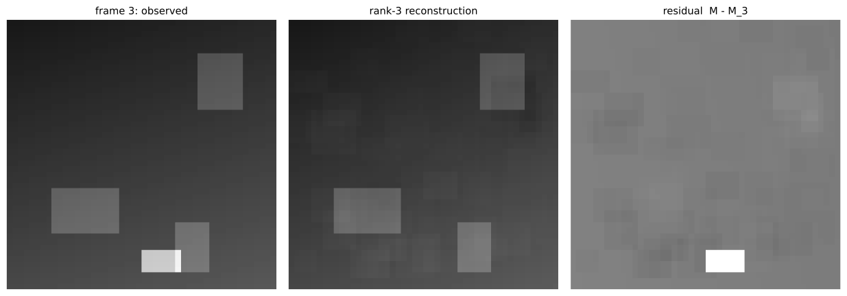

Figure 2

reconstruction error  ||M - M_3||_F / ||M||_F = 0.1675
ghosting error  ||M_3 - B||_F / ||B||_F     = 0.0790

The numbers make the failure concrete. Measured against the true background \mathbf{B}, which the construction knows exactly, the rank-3 reconstruction is off by several percent of the background energy: the rectangles’ energy, roughly one percent of the video’s total, is smeared across the whole reconstruction rather than confined to the pixels it actually occupies. The residual \mathbf{M} - \mathbf{M}_3 is dominated by the rectangles themselves — the SVD leaves the people in the error term exactly where it found them. Truncation cannot tell “structure the model cannot fit” from “structure the model must keep”. The singular values say why: \sigma_1, the background, dwarfs everything else, and a long, slowly decaying tail follows — the outliers smear the spectrum the way chapter 3 described pure noise doing.

The model: \mathbf{M} = \mathbf{L} + \mathbf{S}

The model. Decompose the observed matrix exactly,

\mathbf{M} = \mathbf{L} + \mathbf{S}, \qquad \operatorname{rank}\mathbf{L} \text{ small}, \quad \mathbf{S} \text{ sparse},

and recover the two components from \mathbf{M} alone. Rank and the number of nonzero entries are both combinatorial objectives, so Principal Component Pursuit (PCP; Candès, Li, Ma, and Wright, 2011 ²) replaces them by their convex surrogates: the nuclear norm \lVert \mathbf{L}\rVert_*, the sum of the singular values of \mathbf{L}, for rank, and the entrywise \ell_1 norm \lVert \mathbf{S}\rVert_1 for sparsity. ³ Both are convex, so the relaxation is a tractable optimization problem rather than a combinatorial search:

\boxed{ \min_{\mathbf{L}, \mathbf{S}}\ \lVert \mathbf{L}\rVert_* + \lambda\lVert \mathbf{S}\rVert_1 \quad \text{subject to} \quad \mathbf{L} + \mathbf{S} = \mathbf{M} }

The balance parameter \lambda sets the trade-off between the two penalties. For data whose entries are normalized to [0, 1] — the scale used here — theory selects

\lambda = \frac{1}{\sqrt{\max(m, n)}} = \frac{1}{\sqrt{2304}} \approx 0.021,

and with this choice PCP recovers both components exactly, provided \operatorname{rank}(\mathbf{L}) is small and the support of \mathbf{S} is sufficiently scattered. Exact recovery — not approximately, exactly — is the headline result of robust PCA. The nuclear norm is the convex envelope of rank on the unit spectral-norm ball, and matrix completion is the sibling problem in which entries of \mathbf{M} are missing rather than corrupted.

The algorithm: alternating soft-thresholding

Both penalties are applied by the same scalar operation. The soft-thresholding operator

\operatorname{shrink}(x, \tau) = \operatorname{sign}(x)\, \max(|x| - \tau, 0)

is the proximal operator of \tau\lvert\cdot\rvert: applied entrywise it minimizes \tfrac12\lVert \mathbf{X} - \mathbf{Z}\rVert_F^2 + \tau\lVert \mathbf{Z}\rVert_1 over \mathbf{Z}, and applied to the singular values of a matrix it minimizes the same expression with the nuclear norm in place of \ell_1 — singular-value soft-thresholding. Soft-thresholding is thus the workhorse for both terms of the objective.

The loop below is an augmented-Lagrangian scheme (an ADMM-style iteration ⁴). With penalty parameter \mu and multiplier \mathbf{Y} \in \mathbb{R}^{m \times n}, each pass is:

1. L step — SVD of \mathbf{M} - \mathbf{S} + \mathbf{Y}/\mu, shrink the singular values by 1/\mu;
2. S step — soft-threshold \mathbf{M} - \mathbf{L} + \mathbf{Y}/\mu entrywise at \lambda/\mu;
3. Y update — \mathbf{Y} \leftarrow \mathbf{Y} + \mu(\mathbf{M} - \mathbf{L} - \mathbf{S});
4. \mu update — \mu \leftarrow \min(\rho\mu, \mu_{\max}), so the constraint \mathbf{L} + \mathbf{S} = \mathbf{M} binds ever more tightly.

Iterate until the relative residual \lVert \mathbf{M} - \mathbf{L} - \mathbf{S}\rVert_F / \lVert \mathbf{M}\rVert_F falls below 10^{-5}, with at most 200 passes.

def shrink(X, tau):
    """Entrywise soft-thresholding: prox of tau * ||X||_1."""
    return np.sign(X) * np.maximum(np.abs(X) - tau, 0)

lam = 1.0 / np.sqrt(max(Mmat.shape))    # PCP balance parameter
mu = 1.25 / np.linalg.norm(Mmat, 2)     # augmented-Lagrangian penalty  <1>
rho, mu_max, tol, max_iter = 1.6, mu * 1e7, 1e-5, 200

L = np.zeros_like(Mmat)
S = np.zeros_like(Mmat)
Y = np.zeros_like(Mmat)

residuals = []
for it in range(1, max_iter + 1):
    U, s, Vt = np.linalg.svd(Mmat - S + Y / mu, full_matrices=False)
    L = (U * shrink(s, 1.0 / mu)) @ Vt
    S = shrink(Mmat - L + Y / mu, lam / mu)
    Y = Y + mu * (Mmat - L - S)
    mu = min(rho * mu, mu_max)
    rel_res = np.linalg.norm(Mmat - L - S, "fro") / np.linalg.norm(Mmat, "fro")
    residuals.append(rel_res)
    if rel_res < tol:
        break

print("converged after", it, "iterations, relative residual = %.2e" % rel_res)
print("constraint violation  ||M - L - S||_F = %.2e"
      % np.linalg.norm(Mmat - L - S, "fro"))
print("residual trace:", ", ".join("%.1e" % r for r in residuals))

converged after 13 iterations, relative residual = 3.34e-06
constraint violation  ||M - L - S||_F = 4.46e-04
residual trace: 8.1e-01, 1.8e-01, 1.1e-01, 2.5e-02, 2.1e-02, 1.8e-02, 1.7e-02, 1.8e-03, 9.7e-04, 4.0e-04, 1.2e-04, 2.5e-05, 3.3e-06

Each annotation carries one idea. <1> The penalty \mu starts at 1.25 / \lVert \mathbf{M}\rVert_2, a scale tied to the data, and grows by the factor \rho on every pass. <2> The SVD runs on \mathbf{M} - \mathbf{S} + \mathbf{Y}/\mu: the current mismatch between the two components, nudged by the scaled multiplier. <3> Soft-thresholding the singular values at 1/\mu zeroes every direction below that scale, which is what keeps \mathbf{L} low-rank. <4> Soft-thresholding entrywise at \lambda/\mu classifies each pixel as background or person. <5> The multiplier update is dual ascent: \mathbf{Y} grows along the constraint violation until the constraint binds.

The printed trace shows the relative residual collapsing in 13 iterations: \lVert \mathbf{M} - \mathbf{L} - \mathbf{S}\rVert_F / \lVert \mathbf{M}\rVert_F \approx 3\times 10^{-6}, a few parts per million of the total signal energy. The absolute violation \approx 5\times 10^{-4} pixels of intensity is equally negligible at this scale.

Note

The expensive step is the SVD. On large videos, one replaces the full factorization inside the loop with a truncated or randomized SVD, which computes only the top few singular directions at a fraction of the cost (random projections, then a small exact SVD of the projected matrix); the soft-thresholding then acts on the singular values that survive. This is how PCP scales to megapixel video.

Recovery: background and foreground

The output of the loop splits the video in two. Columns of \mathbf{L} are frames of the recovered background; columns of \mathbf{S} are the foreground. The ground truth is known by construction, so both components can be scored quantitatively and compared with the baseline of the previous section.

fig, axes = plt.subplots(2, 6, figsize=(14, 5.4))
for j, fr in enumerate(frames):
    axes[0, j].imshow(L[:, fr].reshape(size, size), cmap="gray", vmin=0, vmax=1)
    axes[0, j].set_title(f"frame {fr}", fontsize=10)
    axes[0, j].axis("off")
    axes[1, j].imshow(S[:, fr].reshape(size, size), cmap="gray", vmin=0, vmax=1)
    axes[1, j].axis("off")
axes[0, 0].set_ylabel(r"$\mathbf{L}$: background", fontsize=11)
axes[1, 0].set_ylabel(r"$\mathbf{S}$: foreground", fontsize=11)
plt.tight_layout()
plt.show()

nz = S != 0
recall = (nz & (Smat > 0)).sum() / (Smat > 0).sum()
fp = (nz & (Smat == 0)).sum() / (Smat == 0).sum()
print("background error  ||L - B||_F / ||B||_F           = %.2e"
      % (np.linalg.norm(L - Bmat, "fro") / np.linalg.norm(Bmat, "fro")))
print("foreground error  ||S - S_true||_F / ||S_true||_F = %.2e"
      % (np.linalg.norm(S - Smat, "fro") / np.linalg.norm(Smat, "fro")))
print("S support recall: %.4f   false-positive rate: %.6f" % (recall, fp))
print("S nonzero entries: %.2f%%" % (100 * nz.mean()))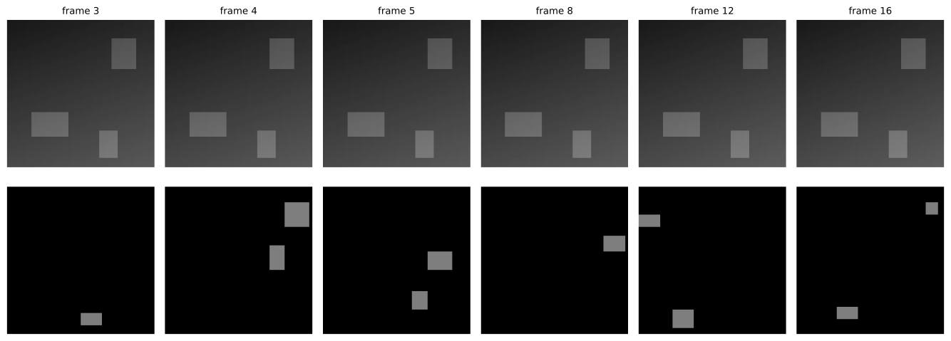

Figure 3

background error  ||L - B||_F / ||B||_F           = 3.54e-06
foreground error  ||S - S_true||_F / ||S_true||_F = 3.97e-06
S support recall: 1.0000   false-positive rate: 0.000000
S nonzero entries: 0.97%

The spectra make the mechanism visible.

s_M = np.linalg.svd(Mmat, compute_uv=False)
s_L = np.linalg.svd(L, compute_uv=False)

fig, ax = plt.subplots(figsize=(7, 4.2))
ax.semilogy(np.arange(1, len(s_M) + 1), s_M, "o-", ms=3.5, lw=1.2,
            label=r"$\sigma_i(\mathbf{M})$")
ax.semilogy(np.arange(1, len(s_L) + 1), np.maximum(s_L, 1e-12), "s-", ms=3.5,
            lw=1.2, label=r"$\sigma_i(\mathbf{L})$")
ax.set_xlabel("index $i$")
ax.set_ylabel(r"$\sigma_i$")
ax.legend(fontsize=11)
plt.tight_layout()
plt.show()

print("sigma(M)[:3] =", np.round(s_M[:3], 3))
print("sigma(L)[:3] =", np.round(s_L[:3], 6))
print("rank(L) =", int(np.sum(s_L > 1e-8 * s_L[0])),
      "   rank(M) =", int(np.sum(s_M > 1e-12 * s_M[0])))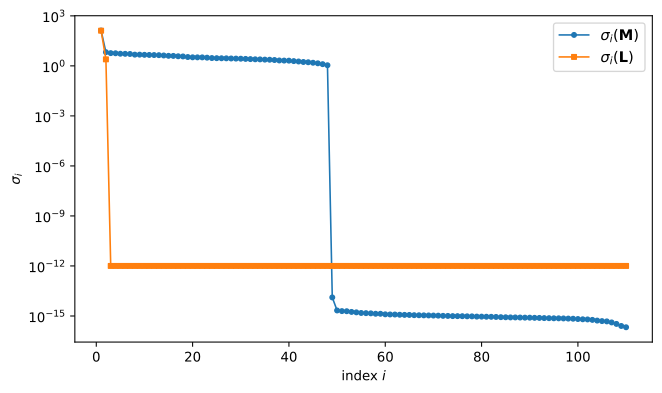

Figure 4

sigma(M)[:3] = [131.545   6.628   5.816]
sigma(L)[:3] = [128.970911   2.461876   0.      ]
rank(L) = 2    rank(M) = 48

The contrast is the lesson. The spectrum of \mathbf{M} has one dominant singular value (the background) and then a long, slowly decaying tail: the rectangles smear energy across dozens of directions, inflating the rank from 2 to a value on the order of the number of frames carrying people. The spectrum of the recovered \mathbf{L} drops to machine zero after the second singular value — exactly the rank of the clean background stack. The outliers were drained into \mathbf{S}, whose support matches the true foreground pixels perfectly (recall 1.00, zero false positives), and the background error \lVert \mathbf{L} - \mathbf{B}\rVert_F / \lVert \mathbf{B}\rVert_F is at machine precision.

Same matrix, same SVD machinery, different objective — and the failure of the previous section is gone. Why? The Frobenius objective of Eckart–Young pays a quadratic price per unit of misfit, so a few large outliers are cheapest when spread thin across many singular vectors; the nuclear-plus-\ell_1 objective pays a linear price per unit, so concentrating the outliers in a sparse component is cheapest. The geometry of the objective, not the data, decides the outcome.

Discussion

The balance parameter. The choice \lambda = 1/\sqrt{\max(m, n)} is derived for data normalized to [0, 1], as here, and tolerates bounded noise: for observations \mathbf{M} = \mathbf{L} + \mathbf{S} + \mathbf{Z} with \lVert \mathbf{Z}\rVert_F \le \delta, the same objective (“stable PCP”) recovers \mathbf{L} and \mathbf{S} up to error proportional to \delta.

Tip

Tuning \lambda in practice. Real data routinely violate the model’s assumptions — noise, correlated outliers, a background that is only approximately static. The formula remains the default, and \lambda becomes the dial: raising it hardens the sparsity requirement and can erode the low-rank component, lowering it lets noise leak into \mathbf{S}. A small grid search with cross-validation is the standard practice.

Connections. Robust PCA is one member of the low-rank-recovery family organized around nuclear-norm minimization: matrix completion recovers \mathbf{L} when entries of \mathbf{M} are missing rather than corrupted, and robust PCA recovers it when entries are corrupted. The two problems share the machinery of this chapter — soft-thresholding, the augmented-Lagrangian loop — and, in the completion case, an extra step that re-inserts the observed entries after each pass. The same L1-sparsity mechanism returns in the next chapter, where it applies to vectors rather than matrices. Applications:

Application	Data matrix \mathbf{M}	Low-rank part \mathbf{L}	Sparse part \mathbf{S}
Surveillance video	frames as columns	static background	moving objects
Face de-noising	aligned face images	clean face manifold	specularities, shadows, occlusions
Collaborative filtering	users \times items ratings	preference structure	rogue ratings
Video post-production	frames	static plate	objects to remove

Summary

Robust PCA decomposes a matrix into a low-rank part and a sparse part by convex relaxation: replace rank with the nuclear norm, replace \ell_0 with \ell_1, and minimize the sum under the exact constraint \mathbf{L} + \mathbf{S} = \mathbf{M}. Both penalties are applied by the same operation — soft-thresholding, entrywise for sparsity and on singular values for rank — inside an augmented-Lagrangian loop that converged in 13 iterations on the synthetic video. Where the Eckart–Young optimum smeared the outliers across the reconstruction, the nuclear-plus-\ell_1 optimum recovered the background and the foreground exactly; only the objective changed, not the SVD machinery.

The sparse half of the story continues in the next chapter. Compressed sensing shows that \ell_1 minimization recovers sparse signals from far fewer measurements than \ell_2 would suggest possible — the same L1-versus-L2 contrast that made robust PCA work, applied to vectors instead of matrices.

Problems

The problems below exercise the PCP machinery of this chapter: the proximal operators behind the two penalties (13-1, 13-2), their numerical verification (13-3, 13-4), and the phase transition of exact recovery (13-5). All random draws use fixed seeds, so every numerical outcome is reproducible.

[P13.1] Soft-thresholding as the proximal operator

The soft-thresholding operator \operatorname{shrink}(x, \tau) = \operatorname{sign}(x)\max(|x| - \tau, 0) is the proximal operator of \tau\lvert\cdot\rvert: for scalar x it is the unique minimizer of \tfrac12(z - x)^2 + \tau\lvert z\rvert over z \in \mathbb{R}.

1. Let f(z) = \tfrac12(z - x)^2 + \tau\lvert z\rvert. Use the subgradient optimality condition 0 \in \partial f(z^*) to show that the minimizer is z^* = \operatorname{shrink}(x, \tau). Treat the three cases x > \tau, x < -\tau, and \lvert x\rvert \le \tau separately.

2. Conclude that entrywise soft-thresholding solves the matrix problem

\boxed{\ \operatorname*{arg\,min}_{\mathbf{Z}} \ \tfrac12\lVert \mathbf{X} - \mathbf{Z}\rVert_F^2 + \tau\lVert \mathbf{Z}\rVert_1 = \operatorname{shrink}(\mathbf{X}, \tau)\ }

applied entrywise, since the objective separates over the entries of \mathbf{Z}.

3. Interpret the case \lvert x\rvert \le \tau, where the minimizer is z^* = 0. What does this mean for the S step of the PCP loop, which thresholds at \lambda/\mu?

[P13.2] Singular-value soft-thresholding and the nuclear norm

The L step of the PCP loop shrinks the singular values of a matrix. This problem proves that this operation is the proximal operator of the nuclear norm.

1. State the von Neumann trace inequality: for \mathbf{X}, \mathbf{Z} \in \mathbb{R}^{m \times n} with singular values \sigma_i(\mathbf{X}) and \sigma_i(\mathbf{Z}),

\langle \mathbf{X}, \mathbf{Z} \rangle \le \sum_{i=1}^{\min(m,n)} \sigma_i(\mathbf{X})\,\sigma_i(\mathbf{Z}),

with equality when \mathbf{Z} shares the singular vectors of \mathbf{X}.

2. Use the inequality to show that the minimizer of \tfrac12\lVert \mathbf{X} - \mathbf{Z}\rVert_F^2 + \tau\lVert \mathbf{Z}\rVert_* over \mathbf{Z} shares the singular vectors of \mathbf{X}, reducing the problem to the scalar problem of Problem 13-1 applied to each singular value.

3. Conclude that the minimizer is \mathbf{Z}^* = \mathbf{U}\operatorname{shrink}(\boldsymbol{\Sigma}, \tau)\mathbf{V}^{\mathsf T}, where \mathbf{X} = \mathbf{U}\boldsymbol{\Sigma}\mathbf{V}^{\mathsf T} is the SVD. Identify this with the L step of the PCP loop.

[P13.3] Verifying the proximal optimality conditions

For a matrix \mathbf{X} and threshold \tau, the matrix \mathbf{Z}^* = \mathbf{U}\operatorname{shrink}(\boldsymbol{\Sigma}, \tau)\mathbf{V}^{\mathsf T} should satisfy the optimality conditions of the nuclear-norm proximal problem: the residual \mathbf{G} = \mathbf{X} - \mathbf{Z}^* must obey \lVert \mathbf{G}\rVert_2 \le \tau and the complementarity identity \langle \mathbf{G}, \mathbf{Z}^*\rangle = \tau\lVert \mathbf{Z}^*\rVert_*.

1. Verify \lVert \mathbf{G}\rVert_2 \le \tau to machine precision.

2. Verify the complementarity identity \langle \mathbf{G}, \mathbf{Z}^*\rangle = \tau\lVert \mathbf{Z}^*\rVert_*.

3. Verify that no perturbed candidate \mathbf{Z}^* + \mathbf{E} achieves a smaller value of f(\mathbf{Z}) = \tfrac12\lVert \mathbf{X} - \mathbf{Z}\rVert_F^2 + \tau\lVert \mathbf{Z}\rVert_*.

The starter code computes \mathbf{Z}^* and prints all three quantities.

import numpy as np

rng = np.random.default_rng(7)
m, n, tau = 20, 15, 0.5
X = rng.standard_normal((m, n))

# SVD soft-thresholding: prox of tau * ||.||_*
U, s, Vt = np.linalg.svd(X, full_matrices=False)
Z = (U * np.maximum(s - tau, 0)) @ Vt
G = X - Z

print("||G||_2 =", np.linalg.norm(G, 2), "  tau =", tau)
print("<G, Z> =", np.sum(G * Z))
print("tau * ||Z||_* =", tau * np.sum(np.linalg.svd(Z, compute_uv=False)))

for _ in range(5):
    E = rng.standard_normal((m, n)) * 0.1
    Zc = Z + E
    f = lambda W: 0.5 * np.sum((X - W) ** 2) + tau * np.sum(np.linalg.svd(W, compute_uv=False))
    print("f(Z + E) - f(Z) =", f(Zc) - f(Z))

||G||_2 = 0.5000000000000208   tau = 0.5
<G, Z> = 23.78494257390281
tau * ||Z||_* = 23.784942573902686
f(Z + E) - f(Z) = 1.5161347976273873
f(Z + E) - f(Z) = 1.6418299760259742
f(Z + E) - f(Z) = 1.6922611098008886
f(Z + E) - f(Z) = 2.0051410095497566
f(Z + E) - f(Z) = 1.7810992669708199

[P13.4] The nuclear norm as a dual norm

The nuclear norm is the dual norm of the spectral norm: \lVert \mathbf{L}\rVert_* = \max_{\lVert \mathbf{Y}\rVert_2 \le 1} \langle \mathbf{Y}, \mathbf{L}\rangle. The maximizer is the SVD alignment \mathbf{Y} = \mathbf{U}\mathbf{V}^{\mathsf T}.

1. Compute \lVert \mathbf{L}\rVert_* as the sum of the singular values of \mathbf{L}.

2. Verify that \mathbf{Y} = \mathbf{U}\mathbf{V}^{\mathsf T} achieves the maximum: \langle \mathbf{L}, \mathbf{U}\mathbf{V}^{\mathsf T}\rangle = \lVert \mathbf{L}\rVert_*.

3. Verify that random \mathbf{Y} with \lVert \mathbf{Y}\rVert_2 = 1 never exceed \lVert \mathbf{L}\rVert_*.

The starter code prints all three quantities.

import numpy as np

rng = np.random.default_rng(11)
m, n = 12, 9
L = rng.standard_normal((m, n))

U, s, Vt = np.linalg.svd(L, full_matrices=False)
nuc = s.sum()
Y = U @ Vt
print("<L, Y> =", np.sum(L * Y), "  ||L||_* =", nuc)

best = -np.inf
for _ in range(2000):
    Yr = rng.standard_normal((m, n))
    Yr = Yr / np.linalg.norm(Yr, 2)
    best = max(best, np.sum(L * Yr))
print("max over random ||Y||_2 = 1:", best)

<L, Y> = 25.121952530205164   ||L||_* = 25.121952530205164
max over random ||Y||_2 = 1: 5.023616457017139

[P13.5] The balance parameter and the phase transition

Challenge. The exact-recovery claim of this chapter has a quantitative edge: recovery succeeds only below a critical sparsity level, and the balance parameter \lambda decides where that level sits. This experiment measures both.

1. For N = 100 and rank r = 5, generate \mathbf{L} = \mathbf{U}\mathbf{V}^{\mathsf T}/\sqrt{N} with Gaussian factors and \mathbf{S} with \pm 1 entries on a random support of fraction \rho_s. For each \rho_s \in \{0.05, 0.10, 0.15, 0.18, 0.20, 0.25\}, run the PCP loop with \lambda = 1/\sqrt{N} and record the relative error \lVert \hat{\mathbf{L}} - \mathbf{L}\rVert_F / \lVert \mathbf{L}\rVert_F.

2. Report the largest \rho_s with error below 10^{-3}, the empirical threshold. Verify that at this \rho_s the recovered \hat{\mathbf{L}} has rank exactly 5: its singular values beyond the fifth should vanish to machine precision.

3. Repeat the sweep with \lambda = 0.5/\sqrt{N} and \lambda = 2/\sqrt{N} on the same instances. Report the largest \rho_s with error below 10^{-3} for each, and explain why the theoretical choice \lambda = 1/\sqrt{\max(m, n)} is the sweet spot.

The starter code defines the PCP loop, generates the instances, and runs the \lambda = 1/\sqrt{N} sweep.

import numpy as np

def pcp(M, lam, mu0, rho=1.6, mu_max=1e7, tol=1e-6, max_iter=500):
    """Augmented-Lagrangian PCP loop (chapter 13)."""
    mu = mu0
    L = np.zeros_like(M); S = np.zeros_like(M); Y = np.zeros_like(M)
    for it in range(max_iter):
        U, s, Vt = np.linalg.svd(M - S + Y / mu, full_matrices=False)
        L = (U * np.maximum(s - 1.0 / mu, 0)) @ Vt
        S = np.sign(M - L + Y / mu) * np.maximum(np.abs(M - L + Y / mu) - lam / mu, 0)
        Y = Y + mu * (M - L - S)
        mu = min(rho * mu, mu_max)
        if np.linalg.norm(M - L - S, "fro") / np.linalg.norm(M, "fro") < tol:
            break
    return L, S

rng = np.random.default_rng(23)
N, r = 100, 5
lam = 1.0 / np.sqrt(N)
rhos = (0.05, 0.10, 0.15, 0.18, 0.20, 0.25)

U = rng.standard_normal((N, r)); V = rng.standard_normal((N, r))
L0 = (U @ V.T) / np.sqrt(N)

instances = []
for rho in rhos:
    S0 = np.zeros((N, N))
    nz = int(rho * N * N)
    idx = rng.choice(N * N, size=nz, replace=False)
    S0.ravel()[idx] = rng.choice([-1.0, 1.0], size=nz)
    instances.append((rho, L0, S0))

def sweep(lam):
    """Run the PCP loop on all instances with a given lambda."""
    for rho, L0, S0 in instances:
        M = L0 + S0
        Lh, Sh = pcp(M, lam, 1.25 / np.linalg.norm(M, 2))
        err = np.linalg.norm(Lh - L0, "fro") / np.linalg.norm(L0, "fro")
        print(f"rho_s={rho:.2f}  rel err = {err:.2e}")

print("lambda = 1/sqrt(N):")
sweep(lam)

lambda = 1/sqrt(N):
rho_s=0.05  rel err = 7.76e-07
rho_s=0.10  rel err = 2.05e-06
rho_s=0.15  rel err = 1.85e-06
rho_s=0.18  rel err = 5.67e-03
rho_s=0.20  rel err = 9.05e-02
rho_s=0.25  rel err = 3.59e-01

Footnotes

1. The name principal component pursuit echoes the sparse-pursuit literature, in which a signal is “pursued” as a small combination of dictionary elements; here the element being pursued is the low-rank component itself.

2. E. J. Candès, X. Li, Y. Ma, and J. Wright, “Robust principal component analysis?”, Journal of the ACM 58(3), 2011.

3. Precisely: on the unit spectral-norm ball the nuclear norm is the convex envelope of the rank function, and on the unit \ell_\infty ball the entrywise \ell_1 norm is the convex envelope of the \ell_0 “norm”.

4. The scheme is the alternating direction method of multipliers on the augmented Lagrangian; each pass costs one SVD of an m \times n matrix, \mathcal{O}(mn\min(m, n)) operations.